Download
1 / 14
140 likes | 298 Views
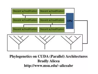
Descent w/modification. Descent w/modification. Descent w/modification. Descent w/modification. CPU. Descent w/modification. Descent w/modification. Phylogenetics on CUDA (Parallel) Architectures Bradly Alicea http://www.msu.edu/~aliceabr. Phylogenetics Introduction.

E N D
Descent w/modification Descent w/modification Descent w/modification Descent w/modification CPU Descent w/modification Descent w/modification Phylogenetics on CUDA (Parallel) Architectures BradlyAlicea http://www.msu.edu/~aliceabr
Phylogenetics Introduction Q: How do we understand evolutionary relationships (e.g. common ancestry, descent with modification)? * use a directed, acyclic graph (from root to last common ancestor to descendents). Tree of Life Viral evolution Within-species diversity
Why Phylogenetics? Answer: inferential tools and data fusion (consensus between different types of data). Phylogeny is the hypothetical relationship between closely-related species. The study of evolution is subject to incomplete/non-uniform sampling: Fossil record Properties of traits Common ancestor A, how did B and C diverge (black box)? Potential answer: trace changes one at a time (one possible set of changes). Diversity
Computational Complexity Sampling of taxa (e.g. species, columns in Mij) + characters (e.g. DNA sequences, rows in Mij) = large # of tree topologies (combinatorics problem). 4 taxa, T = 15 8 taxa, T = 135135 14 taxa, T ~ 7.906 + E12 where n – 1 is # of taxa (rooted case). for n ≥ 3 Unique perfect phylogeny (best evolutionary hypothesis) is NP-hard (for Mij ≥ 10-112), so we use heuristic techniques to approximate answer. 1) Maximum parsimony: nonparametric, best tree is one with least number of unique changes. Minimax method. 2) Maximum likelihood: parametric model estimated from data. Probability distribution for particular tree topologies.
Issues with Existing Methods 1. What methods recover the true tree most often? Maximum Parsimony: gradient descent, lowest scores win (generates “best” trees). Maximum Likelihood: search space pruned using dynamic programming, generates series of “best” subtrees. Four-taxon problem: toy problem for comparing parsimony and likelihood methods. Siddall, Cladistics, 14, 209-220 (1998) 2. What methods are better at exception-handling? 1) Long-branch attraction: when two branches are reported to have same common ancestor but should be phylogenetically distant. 2) Polytomy: when many branches occur at the same time (rapid speciation, lack of resolution).
Example #1 Suchard and Rambaut, Many-core algorithms for statistical phylogenetics. Bioinformatics, 25(11), 1370-1376. • Bayesian model (e.g. Maximum Likelihood): • * 62 mitochondrial genomes, carnivores • (60 state codon model). • * 90-fold increase over CPU models. • * parallelization strategy = Felsenstein’s “peeling” algorithm (1981). Nucleotide-based model: each base (A, C, G, T) serves as a character. * 4 possible states per character, total # characters = total # of nucleotide positions sampled (n). Codon-based model: each combination of three nucleotides (e.g. ACT, TCT, GAG) serves as a character. * 64 possible states (43) per character, total # characters = n / 3.
Model and Approach to Likelihood Fu = {Furcs} matrix of size R x C x S t2 alignment columns t1 “Peeling” procedure rate of state transition (e.g. mutation) t0 * element Fus = probability that node u is in state s. Travel upward through tree, compute forward likelihoods for each internal node u. Forward likelihoods, t1 and t2 Finite-time transition probabilities, t1 and t2 When data areunambiguous, algorithm runs in O(RCS2) time.
Many-core Implementation Many-core implementation: * for each node u recursively (every u, c, s) – distribute so that each (r, c, s) entry executes its own thread. * for each (r, c, s), small portion of code dedicated to computing Furcs. * previous approach to parallelization: partition columns into conditionally-independent blocks, distribute blocks across separate cores. Four vectors calculated: 1-2) Reading forward likelihoods of child nodes {Fϕ(bn)rcj}. 3-4) finite-time transition probability matrices {Psj(r)(tbn)}. GPU coalesces memory read/writes of 16 consecutive threads into single transaction. Zero-padding used to deal with stop codons, other zero-probability states.
CPU vs. GPU MCMC (Markov Chain Monte Carlo)-based resampling techniques implemented in single (32-bit) and double (64-bit) precision. * in both cases, large speedup vs. CPU. Important scaling dimensions: • state-space size (S). For nucleotides (S= 4), speedup using GPU becomes more modest. 2) alignment columns (C) – very small, large C values show limited benefit on GPU. 3) number of taxa (N) – performance saturates on GPU for larger values.
Reconstructed Tree, GPU Tree reconstructions form “clades”, or sets of related taxa. Clade membership = statistical support: * maximum parsimony: bootstrap values. * maximum likelihood: posterior probabilities. Outgroup: helps to order the tree topology (distantly-related species). Molecular clock: hypothesized rate of change for specific gene (can be a constant). Clades should be nested: Clade A = A U B. Clade B Clade A
Example #2 Pratas et al, Fine-grained parallelism using multi-core, Cell/BE, and GPU systems: accelerating the phylogenetic likelihood function. International Conference on Parallel Processing, 9-17 (2009). • Implemented MrBayes, a commonly-used program for phylogenomics, on multi-core CPU and GPGPU. • * fine-grained parallelism = very small threads. • * compute phylogenetic likelihood function (PLF) on known phylogeny, ultimate goal is benchmarking rather than reconstruction. • * can GPU improve inferential power of ML model? • Goal is to speed-up computation of the PLF in parallel, so that in application search time among a large amount of potential tree topologies can be minimized.
Rooting/Likelihood Construction MrBayes (Bayesian inference), Maximum Likelihood. Phylogenetic Likelihood Functions (PLF) require substitution, conditional probability information. * estimate branch lengths and parameters of nucleotide substitution model (matrix Q, Figure 2). * three main functions: CondLikeDown, CondLikeRoot, CondLikeScaler. PLF = independent for loops, load depends on sequence length (m) and number of discrete rates (r). * Down, Root - multiply likelihood vector elements by substitution matrix for each discrete rate (16 inner products required). Scaler - properly scale computation.
Partitioning Data for GPU Phylogenomic data example: 1500 genes, ML analysis = 2+E06. Efficient use of the GPU: Number of threads must be maximized using one of two approaches: 1) direct parallelization (use group of threads in parallel, requires large number of synchronization points and conditional statements). 2) parallelize work at the likelihood vector entry level. * calculation of each vector entry assigned to independent threads (avoid overhead). Second approach: less concurrency and completely independent threads.
Final Issue: Scalability Scalability: input data characterized by leaves (taxa) and columns (characters): * leaves (number of calls to the PLF), columns (size of data computed in loops). * multi-core CPU architectures: efficiency of fine-grained parallelism depends on number of cores sharing resources (intra-chip, cross-core communication). * GPU: speedup as dataset increases (up to 20-50K columns). Speedup increases with computational intensity (GPU optimized for executing small parallel threads). GPU benefit realized when computation-to-data ratio is high. GPU vs. CPU: neither method is uniformly superior: * largest overhead for GPU: transfer of data (overall, need for better data sharing and more efficient communication mechanisms). * parallelization time (programming) for MrBayes: 1/2 day for multi-core CPU vs. 2 days on GPU. CPU wins on this count. * both multi-core CPU and GPU reduce amount of time consumed in the execution of the PLF. For baseline, 90%. Multi-core CPU = 10-15% vs. GPU = 5-10%. GPU wins on this count.