Download
1 / 113
1.18k likes | 1.68k Views
Basic Genetics. The First International Workshop on Statistical & Computational Genetics. August 2—9, 2009. (1) Mendelian genetics How does a gene transmit from a parent to its progeny (individual)? (2) Population genetics

E N D
Basic Genetics The First International Workshop on Statistical & Computational Genetics August 2—9, 2009
(1) Mendelian genetics How does a gene transmit from a parent to its progeny (individual)? (2) Population genetics How is a gene segregating in a population (a group of individuals)? (3) Quantitative genetics How is gene segregation related with the phenotype of a character? (4) Molecular genetics What is the molecular basis of gene segregation and transmission? (5) Developmental genetics (6) Epigenetics (genetic imprinting)
Mendelian Genetics Probability Population GeneticsStatistics Quantitative genetics Molecular Genetics Statistical Genetics Mathematics with biology (our view) Cutting-edge research into the interface among genetics, evolution and development (Evo-Devo) Wu, R. L. and M. Lin, Functional mapping of complex traits. Nature Reviews Genetics.
Mendel’s Laws Mendel’s first law • There is a gene with two alleles on a chromosome location (locus) • These alleles segregate during the formation of the reproductive cells, thus passing into different gametes Diploid Gene A A| a | Centromere A | a | Probability ½ ½ Gamete Gamete A pair of chromosomes
Mendel’s second law • There are two or more pairs of genes on different chromosomes • They segregate independently (partially correct) Diploid A|a|, B|b| A|, B| A|, b| a|, B| a|, b| Probability¼ ¼ ¼ ¼ Four two-gene gametes
Linkage (exception to Mendel’s second law) • There are two or more pairs of genes located on the same chromosome • They can be linked or associated (the degree of association is described by the recombination fraction) High linkage Low linkage A A B B
How the linkage occurs? – consider two genes A andB 1 2 3 4 A a A A a a A a A a A a A a B b B B b b B B b b B B b b Stage 1: A pair of chromosomes, one from the father and the other from the mother Stage 2: Each chromosome is divided into two sister chromatids Stage 3: Non-sister chromatids crossover Stage 4: Meiosis generates four gametes AB, aB, Ab and ab – Nonrecombinants (AB and ab) and Recombinants (aB and Ab)
How to measure the linkage? – based on a design Parents AABB × aabb Gamete AB ab F1 AaBb × aabb Gamete AB Ab aB ab ab Backcross AaBb Aabb aaBb aabb Observations n1 n2 n3 n4 Gamete type Non-recom/ Recom/ Recom/ Non-recom/ Parental Non-parental Non-parental Parental Define the proportion of the recombinant gametes over the total gametes as the recombination fraction (r) between two genes A and B r = (n2+n3)/(n1+n2+n3+n4)
Several concepts Genotype and Phenotype • Locus (loci), chromosomal location of a gene • Allele (A, a), a copy of gene • Dominant allele, one allele whose expression inhibits the expression of its alternative allele • Recessive allele (relative to dominant allele) • Dominant gene (AA and Aa are not distinguishable, denoted by A_) • Codominant gene (AA, Aa and aa are mutually distinguishable) • Genotype (AA, Aa or aa) • Homozygote (AA or aa) • Heterozygote (Aa) • Phenotype: trait value
Chromosome and Meiosis • Chromosome: Rod-shaped structure made of DNA • Diploid (2n): An organism or cell having two sets of chromosomes or twice the haploid number • Haploid (n): An organism or cell having only one complete set of chromosomes • Gamete: Reproductive cells involved in fertilization. The ovum is the female gamete; the spermatozoon is the male gamete. • Meiosis: A process for cell division from diploid to haploid (2n n) (two biological advantages: maintaining chromosome number unchanged and crossing over between different genes) • Crossover: The interchange of sections between pairing homologous chromosomes during meiosis • Recombination, recombinant, recombination fraction (rate, frequency): The natural formation in offspring of genetic combinations not present in parents, by the processes of crossing over or independent assortment.
Molecular markers • Genetic markers are DNA sequence polymorphisms that show Mendelian inheritance • Marker types - Restriction fragment length polymorphism (RFLP) - Amplified fragment length polymorphism (AFLP) - Simple sequence repeat (SSR) - Single nucleotide polymorphism (SNP)
Population Genetics • Different copies of a gene are called alleles; for example A and a at gene A; • These alleles form three genotypes, AA, Aa and aa; • The allele (or gene) frequency of an allele is defined as the proportion of this allele among a group of individuals; • Accordingly, the genotype frequency is the proportion of a genotype among a group of individuals
Calculations of allele frequencies and genotype frequencies Genotypes Counts Estimates genotype frequencies AA 224 PAA = 224/294 = 0.762 Aa 64 PAa = 64/294 = 0.218 aa 6 Paa = 6/294 = 0.020 Total 294 PAA + PAa + Paa = 1 Allele frequencies pA = (2214+64)/(2294)=0.871, pa = (26+64)/(2294)=0.129, pA + pa = 0.871 + 0.129 = 1 Expected genotype frequencies AA pA2 = 0.8712 = 0.769 Aa 2pApa = 2 0.871 0.129 = 0.224 aa pa2 = 0.1292 = 0.017
Genotypes Counts Estimates of genotype freq. AA nAA PAA = nAA/n Aa nAa PAa = nAa/n aa naa Paa = naa/n Total n PAA + PAa + Paa = 1 Allele frequencies pA = (2nAA + nAa)/2n pa = (2naa + nAa)/2n Standard error of the estimate of the allele frequency Var(pA) = pA(1 - pA)/2n
The Hardy-Weinberg Law • In the Hardy-Weinberg equilibrium (HWE), the relative frequencies of the genotypes will remain unchanged from generation to generation; • As long as a population is randomly mating, the population can reach HWE from the second generation; • The deviation from HWE, called Hardy-Weinberg disequilibrium (HWD), results from many factors, such as selection, mutation, admixture and population structure…
Mendelian inheritance at the individual level (1) Make a cross between two individual parents (2) Consider one gene (A) with two alleles A and a AA, Aa, aa Thus, we have a total of nine possible cross combinations: Cross Mendelian segregation ratio 1. AA AA AA 2. AA Aa ½AA + ½Aa 3. AA aa Aa 4. Aa AA ½AA + ½Aa 5. Aa Aa ¼AA + ½Aa + ¼aa 6. Aa aa ½Aa + ½aa 7. aa AA Aa 8. aa Aa ½Aa + ½aa 9. aa aa aa
Mendelian inheritance at the population level • A population, a group of individuals, may contain all these nine combinations, weighted by the mating frequencies. • Genotype frequencies: AA, PAA; Aa, PAa; aa, Paa Cross Mating freq. (t) Mendelian segreg. ratio (t+1) AA Aa aa 1. AA AA PAA(t)PAA(t) 1 0 0 2. AA Aa PAA(t)PAa(t) ½ ½ 0 3. AA aa PAA(t)Paa(t) 0 1 0 4. Aa AA PAa(t)PAA(t) ½ ½ 0 5. Aa Aa PAa(t)PAa(t) ¼ ½ ¼ 6. Aa aa PAa(t)Paa(t) 0 ½ ½ 7. aa AA Paa(t)PAA(t) 0 1 0 8. aa Aa Paa(t)PAa(t) 0 ½ ½ 9. aa aa Paa(t)Paa(t) 0 0 1
PAA(t+1) = 1[PAA(t)]2 + ½ 2[PAA(t)PAa(t)] + ¼[PAa(t)]2 = [PAA(t) + ½PAa(t)]2 Similarly, we have Paa(t+1) = [Paa(t) + ½PAa(t)]2 PAa(t+1) = 2[PAA(t) + ½PAa(t)][Paa(t) + ½PAa(t)] Therefore, we have [PAa(t+1)]2 = 4PAA(t+1)Paa(t+1) Furthermore, if random mating continues, we have PAA(t+2) = [PAA(t+1) + ½PAa(t+1)]2 = PAA(t+1) PAa(t+2) = 2[PAA(t+1) + ½PAa(t+1)][Paa(t+1) + ½PAa(t+1)] = PAa(t+1) Paa(t+2) = [Paa(t+1) + ½PAa(t+1)]2 = Paa(t+1)
Concluding remarks A population with [PAa(t+1)]2 = 4PAA(t+1)Paa(t+1) is said to be in Hardy-Weinberg equilibrium (HWE). The HWE population has the following properties: (1) Genotype (and allele) frequencies are constant from generation to generation, (2) Genotype frequencies = the product of the allele frequencies, i.e., PAA = pA2, PAa = 2pApa, Paa = pa2 For a population at Hardy-Weinberg disequilibrium (HWD), we have • PAA = pA2 + D • PAa = 2pApa – 2D • Paa = pa2 + D The magnitude of D determines the degree of HWD. • D = 0 means that there is no HWD. • D has a range of max(-pA2 , -pa2) D pApa
Chi-square test for HWE • Whether or not the population deviates from HWE at a particular locus can be tested using a chi-square test. • If the population deviates from HWE (i.e., Hardy-Weinberg disequilibrium, HWD), this implies that the population is not randomly mating. Many evolutionary forces, such as mutation, genetic drift and population structure, may operate.
Example 1 AA Aa aa Total Obs 224 64 6 294 Exp n(pA2) = 222.9 n(2pApa) = 66.2 n(pa2) = 4.9 294 Test statistics 2 = (obs – exp)2 /exp = (224-222.9)2/222.9 + (64-66.2)2/66.2 + (6-4.9)2/4.9 = 0.32 is less than 2df=1 ( = 0.05) = 3.841 Therefore, the population does not deviate from HWE at this locus. Why the degree of freedom = 1? Degree of freedom = the number of parameters contained in the alternative hypothesis – the number of parameters contained in the null hypothesis. In this case, df = 2 (pA or pa and D) – 1 (pA or pa) = 1
Example 2 AA Aa aa Total Obs 234 36 6 276 Exp n(pA2) n(2pApa) n(pa2) = 230.1 = 43.8 = 2.1 276 Test statistics 2 = (obs – exp)2/exp = (234-230.1)2/230.1+(36-43.8)2/43.8+(6-2.1)2/2.1 = 8.8 is greater than 2df=1 ( = 0.05) = 3.841 Therefore, the population deviates from HWE at this locus.
Linkage disequilibrium • Consider two loci, A and B, with alleles A, a and B, b, respectively, in a population • Assume that the population is at HWE • If the population is at Hardy-Weinberg equilibrium, we have Gene A Gene B AA: PAA = pA2 BB: PBB = pB2 Aa: PAa = 2pApa Bb: PBb = 2pBpb aa: Paa = pa2 bb: Pbb = pb2 PAA+PAa+Paa = 1 PBB+PBb+Pbb=1 pA + pa = 1 pB + pb = 1
But the population is at Linkage Disequilibrium (for a pair of loci). Then we have • Two-gene haplotype AB: pAB = pApB + DAB • Two-gene haplotype Ab: pAb = pApb + DAb • Two-gene haplotype aB: paB = papB + DaB • Two-gene haplotype ab: pab = papb + Dab pAB+pAb+paB+pab = 1 Dij is the coefficient of linkage disequilibrium (LD) between the two genes in the population. The magnitude of D reflects the degree of LD. The larger D, the stronger LD.
pA = pAB+pAb = pApB + DAB + pApb + DAb = pA+DAB+DAb DAB = -DAb pB = pAB+paB = pB+DAB+DaB DAB = -DaB pb = pAb+pab = pb+DaB+Dab Dab = -DaB Finally, we have DAB = -DAb = -DaB = Dab = D. Re-write four two-gene haplotypes • AB: pAB = pApB + D • Ab: pAb = pApb – D • aB: paB = papB – D • ab: pab = papb + D D = pABpab - pAbpaB D = 0 the population is at the linkage equilibrium
How does D transmit from one generation (1) to the next (2)? D(2) = (1-r)1 D(1) … D(t+1) = (1-r)t D(1) t, D(t+1) r
Proof to D(t+1) = (1-r)1 D(t) • The four gametes randomly unite to form a zygote. The proportion 1-r of the gametes produced by this zygote are parental (or nonrecombinant) gametes and fraction r are nonparental (or recombinant) gametes. A particular gamete, say AB, has a proportion (1-r) in generation t+1 produced without recombination. The frequency with which this gamete is produced in this way is (1-r)pAB(t). • Also this gamete is generated as a recombinant from the genotypes formed by the gametes containing allele A and the gametes containing allele B. The frequencies of the gametes containing alleles A or B are pA(t) and pB(t), respectively. So the frequency with which AB arises in this way is rpA(t)pB(t). • Therefore the frequency of AB in the generation t+1 is pAB(t+1) = (1-r)pAB(t) + rpA(t)pB(t) By subtracting is pA(t)pB(t) from both sides of the above equation, we have D(t+1) = (1-r)1 D(t) Whence D(t+1) = (1-r)t D(1)
Estimate and test for LD Two markers A and B: Four haplotypes Frequencies AB pAB Ab pAb aB paB ab pab
Data Structure and expected genotype frequencies (assuming a random mating) BB (PBB) Bb (PBb) bb (Pbb) _______________________________________________________________________________________ AA (PAA) n22 n21 n20 pAB2 2pABpAb pAb2 Aa (PAa) n12 n11 n10 2pABpaB 2(pABpab+pAbpaB) 2pAbpab aa (Paa) n02 n01 n00 paB2 2paBpab pab2 ________________________________________________________________________________________ Multinomial pdf H1: D 0 log f(pij|n) = log n!/(n22!…n00!) + n22 log pAB2 + n21log (2pABpAb) + n20 log pAb2 + … Estimate pAB, pAb, paB (pab = 1-pAB-pAb-paB) pA, pB, D H0: D = 0 log f(pi,pj|n) = log n!/(n22!…n00!) + n22log(pApB)2 + n21log(2pA2pBpb)+n20log(pApb)2 + … Estimate pA and pB.
H1BB (PBB) Bb (PBb) bb (Pbb) AA (PAA) Freq pAB2 2pABpAb pAb2 Obs n22 n21 n20 #pAB 2 1 0 #pAb 0 1 2 #paB 0 0 0 #pab 0 0 0 Aa (PAa) Freq 2pABpaB 2(pABpab+pAbpaB) 2pAbpab Obs n12 n11 n10 #pAB 1 =(pABpab)/ (pABpab+pAbpaB) 0 #pAb 0 1-= (pAbpaB)/ (pABpab+pAbpaB) 1 #paB 1 1-=(pAbpaB)/ (pABpab+pAbpaB) 0 #pab 0 =(pABpab)/ (pABpab+pAbpaB) 1 aa (Paa) Freq paB2 2paBpab pab2 Obs n02 n01 n00 #pAB 0 0 0 #pAb 0 0 0 #paB 2 1 0 #pab 0 1 2
The estimator of haplotype frequencies • pAB = 1/(2n)[2n22 + (n21+n12) + n11] (1) • pAb = 1/(2n)[2n20 + (n21+n10) + (1-)n11] (2) • paB = 1/(2n)[2n02 + (n01+n12) + (1-)n11] (3) • pab = 1/(2n)[2n00 + (n10+n01) + n11] (4) • EM algorithm • E step: Calculate • M step: Calculate pAB, …, pab using equations (1) - (4) • Specific estimating steps • Give initiate values for pAB(1)= pAb(1) = paB(1) = pa(1)= 0.5; • Calculate (1) =(pAB(1)pab(1))/ (pAB(1)pab(1) + pAb(1)paB(1)); • 3. Calculate pAB(2),pAb(2),paB(2),pab(2); • Repeat steps 2 and 3 until the estimates of haplotype frequencies converge. The values at the convergence are the MLEs.
What is the convergence? |pAB(t+1) - pAB(t)| < a very small value |pAb(t+1) - pAb(t)| < a very small value |paB(t+1) - paB(t)| < a very small value |pab(t+1) - pab(t)| < a very small value For example, this very small value is e-8
H0BB (PBB) Bb (PBb) bb (Pbb) AA (PAA) Freq pA2pB2 2pA2pBpb pA2pb2 Obs n22 n21 n20 #pA 2 2 2 #pa 0 0 0 #pB 2 1 0 #pb 0 1 2 Aa (PAa) Freq 2pApapB2 4pApapBpb 2pApapb2 Obs n12 n11 n10 #pA 1 1 1 #pa 1 1 1 #pB 2 1 0 #pb 0 1 2 aa (Paa) Freq pa2 pB2 2pa2pBpb pa2pb2 Obs n02 n01 n00 #pA 0 0 0 #pa 2 2 2 #pB 2 1 0 #pb 0 1 2
The estimator of allele frequencies: pA = 1/(2n)[2(n22 + n21 + n20) + (n12 + n11 + n10)] pa = 1/(2n)[2(n02 + n01 + n00) + (n12 + n11 + n10)] pB = 1/(2n)[2(n22 + n12 + n02) + (n21 + n11 + n01)] pb = 1/(2n)[2(n20 + n10 + n00) + (n21 + n11 + n01)] No EM algorithm is needed to obtain the MLEs of these allele frequencies
Plugging in the MLEs into the likelihood functions under the two hypotheses: H1: D 0 log L1 = log n!/(n22!…n00!) + n22 log pAB2 + n21log (2pABpAb) + n20 log pAb2 + … H0: D = 0 log L0 = log n!/(n22!…n00!) + n22log(pApB)2 +n21log(2pA2pBpb)+n20log(pApb)2 + … LR = -2(log L0 – log L1) ~ 2(df=1,0.05) = 3.841
Other approaches for testing LD: Chi-square Test Test statistic 2 = 2nD2/(pApapBpb) is compared with the critical threshold value obtained from the chi-square table 2df=1 (0.05). n is the number of individuals in the population. If 2 < 2df=1 (0.05), this means that D is not significantly different from zero and that the population under study is in linkage equilibrium. If 2 > 2df=1 (0.05), this means that D is significantly different from zero and that the population under study is in linkage disequilibrium.
Example (1) Two genes A with allele A and a, B with alleles B and b, whose population frequencies are denoted by pA, pa (=1- pA) and pB, pb (=1- pb), respectively (2) These two genes are associated with each other, having the coefficient of linkage disequilibrium D Four gametes are observed as follows: Gamete AB Ab aB ab Total Obs 474 611 142 773 2n=2000 Gamete frequency pAB pAb paB pab =474/2000 =611/2000 =142/2000 =773/2000 =0.237 =0.305 =0.071 =0.386 1
Estimates of allele frequencies pA = pAB + pAb = 0.237 + 0.305 = 0.542 pa = paB + pab = 0.071 + 0.386 = 0.458 pB = pAB + paB = 0.237 + 0.071 = 0.308 pb = pAb + pab = 0.305 + 0.386 = 0.692 The estimate of D D = pABpab –pAbpaB = 0.237 0.386 – 0.305 0.071 = 0.0699 Test statistics 2 = 2nD2/ (pApapBpb) =210000.06992/(0.5420.4580.3080.692) = 184.78 is greater than 2df=1 (0.05) = 3.841. Therefore, the population is in linkage disequilibrium at these two genes under consideration.
2 can also be calculated by Gamete AB Ab aB ab Total Obs 474 611 142 773 2n=2000 Exp 2n(pApB) 2n(pApb) 2n(papB) 2n(papb) =334.2 =750.8 =281.8 =633.2 2000 2 = (obs – exp)2 /exp = (474-334.2)2/334.2 + (611-750.8)2/750.8 + (142-281.8)2/281.8 + (773-633.2)2/633.2 = 184.78 = 2nD2/ (pApapBpb)
Measures of linkage disequilibrium • D, which has a limitation that its value depends on the allele frequencies D = 0.02 is considered to be • large for two genes each with diverse allele frequencies, e.g., pA = pB = 0.9 vs. pa = pb = 0.1 • small for two genes each with similar allele frequencies, e.g., pA = pB = 0.5 vs. pa = pb = 0.5
To make a comparison between gene pairs with different allele frequencies, we need a new normalized measure. The range of LD is max(-pApB, -papb) D min(pApb, papB) The normalized LD (Lewontin 1964) is defined as D' = D/ Dmax, where Dmax is the maximum that D can have, which is Dmax = max(-pApB, -papb) if D < 0, or min(pApb, papB) if D > 0. For the above example, we have D' = 0.0699/min(pApb, papB) = 0.0699/min(0.375, 0.141) = 0.496
(3) Linkage disequilibrium measured as the correlation between the A and B alleles R = D/(pApapBpb), r: [-1, 1] Note: 2= 2nR2 follows the chi-square distribution with df = 1 under the null hypothesis of D = 0. For the above example, we have R = 0.0699/(pApbpapB) = 0.3040.
Application of LD analysis D(t+1) = (1-r)tD(1), This means that when the population undergoes random mating, the LD decays exponentially in a proportion related to the recombination fraction. (1) Population structure and evolution Estimating D, D' and R the mating history of population The larger the D’ and R estimates, the more likely the population in nonrandom mating, the more likely the population to have a small size, the more likely the population to be affected by evolutionary forces.
Human origin studies based on LD analysis Reich, D. E., M. Cargill, S. Bolk, J. Ireland, P. C. Sabeti, D. J. Richter, T. Lavery, R. Kouyoumjian, S. F. Farhadian, R. Ward and E. S. Lander, 2001 Linkage disequilibrium in the human genome. Nature 411: 199-204. Dawson, E., G. R. Abecasis, S. Bumpstead, Y. Chen et al. 2002 A first-generation linkage disequilibrium map of human chromosome 22. Nature 418: 544-548.
LD curve for Swedish and Yoruban samples. To minimize ascertainment bias, data are only shown for marker comparisons involving the core SNP. Alleles are paired such that D' > 0 in the Utah population. D' > 0 in the other populations indicates the same direction of allelic association and D' < 0 indicates the opposite association. a, In Sweden, average D' is nearly identical to the average |D'| values up to 40-kb distances, and the overall curve has a similar shape to that of the Utah population (thin line in a and b). b, LD extends less far in the Yoruban sample, with most of the long-range LD coming from a single region, HCF2. Even at 5 kb, the average values of |D'| and D' diverge substantially. To make the comparisons between populations appropriate, the Utah LD curves are calculated solely on the basis of SNPs that had been successfully genotyped and met the minimum frequency criterion in both populations (Swedish and Yoruban) (Reich,te al. 2001)
(2) Fine mapping of disease genes The detection of LD may imply that the recombination fraction between two genes is small and therefore closer (given the assumption that t is large).
Human Chromosomes Male Xy Xy FemaleXXXXXXy Daughter Son