Download
1 / 67
700 likes | 974 Views
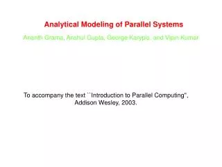
Analytical Modeling of Parallel Systems. Ananth Grama, Anshul Gupta, George Karypis, and Vipin Kumar. To accompany the text ``Introduction to Parallel Computing'', Addison Wesley, 2003. 67 Slides. Topic Overview. Sources of Overhead in Parallel Programs

E N D
Analytical Modeling of Parallel Systems Ananth Grama, Anshul Gupta, George Karypis, and Vipin Kumar To accompany the text ``Introduction to Parallel Computing'', Addison Wesley, 2003. 67 Slides
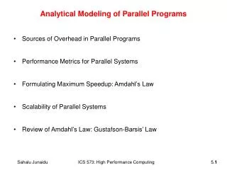
Topic Overview • Sources of Overhead in Parallel Programs • Performance Metrics for Parallel Systems • Effect of Granularity on Performance • Scalability of Parallel Systems • Minimum Execution Time and Minimum Cost-Optimal Execution Time • Asymptotic Analysis of Parallel Programs • Other Scalability Metrics
Analytical Modeling - Basics • A sequential algorithm is evaluated by its runtime (in general, asymptotic runtime as a function of input size). • The asymptotic runtime of a sequential program is identical on any serial platform. • The parallel runtime of a program depends on the input size, the number of processors, and the communication parameters of the machine. • An algorithm must therefore be analyzed in the context of the underlying platform. • A parallel system is a combination of a parallel algorithm and an underlying platform.
Analytical Modeling - Basics • A number of performance measures are intuitive. • Wall clock time - the time from the start of the first processor to the stopping time of the last processor in a parallel ensemble. But how does this scale when the number of processors is changed of the program is ported to another machine altogether? • How much faster is the parallel version? This begs the obvious followup question - whats the baseline serial version with which we compare? Can we use a suboptimal serial program to make our parallel program look • Raw FLOP count - What good are FLOP counts when they dont solve a problem?
Sources of Overhead in Parallel Programs • If I use two processors, shouldnt my program run twice as fast? • No - a number of overheads, including wasted computation, communication, idling, and contention cause degradation in performance. The execution profile of a hypothetical parallel program executing on eight processing elements. Profile indicates times spent performing computation (both essential and excess), communication, and idling.
Sources of Overheads in Parallel Programs • Interprocess interactions: Processors working on any non-trivial parallel problem will need to talk to each other. • Idling: Processes may idle because of load imbalance, synchronization, or serial components. • Excess Computation: This is computation not performed by the serial version. This might be because the serial algorithm is difficult to parallelize, or that some computations are repeated across processors to minimize communication.
Performance Metrics for Parallel Systems: Execution Time • Serial runtime of a program is the time elapsed between the beginning and the end of its execution on a sequential computer. • The parallel runtime is the time that elapses from the moment the first processor starts to the moment the last processor finishes execution. • We denote the serial runtime by TS and the parallel runtime by TP .
Performance Metrics for Parallel Systems: Total Parallel Overhead • Let Tall be the total time collectively spent by all the processing elements. • TS is the serial time. • Observe that Tall - TS is then the total time spend by all processors combined in non-useful work. This is called the total overhead. • The total time collectively spent by all the processing elements Tall = p TP (p is the number of processors). • The overhead function (To) is therefore given by To = p TP - TS (1)
Performance Metrics for Parallel Systems: Speedup • What is the benefit from parallelism? • Speedup (S) is the ratio of the time taken to solve a problem on a single processor to the time required to solve the same problem on a parallel computer with p identical processing elements.
Performance Metrics: Example • Consider the problem of adding n numbers by using n processing elements. • If n is a power of two, we can perform this operation in log n steps by propagating partial sums up a logical binary tree of processors.
Performance Metrics: Example Computing the globalsum of 16 partial sums using 16 processing elements . Σji denotes the sum of numbers with consecutive labels from i to j.
Performance Metrics: Example (continued) • If an addition takes constant time, say, tc and communication of a single word takes time ts + tw, we have the parallel time TP = Θ (log n) • We know that TS = Θ (n) • Speedup S is given by S = Θ (n /log n)
Performance Metrics: Speedup • For a given problem, there might be many serial algorithms available. These algorithms may have different asymptotic runtimes and may be parallelizable to different degrees. • For the purpose of computing speedup, we always consider the best sequential program as the baseline.
Performance Metrics: Speedup Example • Consider the problem of parallel bubble sort. • The serial time for bubblesort is 150 seconds. • The parallel time for odd-even sort (efficient parallelization of bubble sort) is 40 seconds. • The speedup would appear to be 150/40 = 3.75. • But is this really a fair assessment of the system? • What if serial quicksort only took 30 seconds? In this case, the speedup is 30/40 = 0.75. This is a more realistic assessment of the system.
Performance Metrics: Speedup Bounds • Speedup can be as low as 0 (the parallel program never terminates). • Speedup, in theory, should be upper bounded by p - after all, we can only expect a p-fold speedup if we use times as many resources. • A speedup greater than p is possible only if each processing element spends less than time TS / p solving the problem. • In this case, a single processor could be timeslided to achieve a faster serial program, which contradicts our assumption of fastest serial program as basis for speedup.
Performance Metrics: Superlinear Speedups One reason for superlinearity is that the parallel version does less work than corresponding serial algorithm. Searching an unstructured tree for a node with a given label, `S', on two processing elements using depth-first traversal. The two-processor version with processor 0 searching the left subtree and processor 1 searching the right subtree expands only the shaded nodes before the solution is found. The corresponding serial formulation expands the entire tree. It is clear that the serial algorithm does more work than the parallel algorithm.
Performance Metrics: Superlinear Speedups • Resource-based superlinearity: The higher aggregate cache/memory bandwidth can result in better cache-hit ratios, and therefore superlinearity. • Example: A processor with 64KB of cache yields an 80% hit ratio. If two processors are used, since the problem size/processor is smaller, the hit ratio goes up to 90%. Of the remaining 10% access, 8% come from local memory and 2% from remote memory. • If DRAM access time is 100 ns, cache access time is 2 ns, and remote memory access time is 400ns, this corresponds to a speedup of 2.43!
Performance Metrics: Efficiency • Efficiency is a measure of the fraction of time for which a processing element is usefully employed • Mathematically, it is given by = (2) • Following the bounds on speedup, efficiency can be as low as 0 and as high as 1.
Performance Metrics: Efficiency Example • The speedup of adding numbers on processors is given by • Efficiency is given by = =
Parallel Time, Speedup, and Efficiency Example Consider the problem of edge-detection in images. The problem requires us to apply a 3x 3template to each pixel. If each multiply-add operation takes time tc, the serial time for an n x n image is given by TS= tcn2. Example of edge detection: (a) an 8 x 8 image; (b) typical templates for detecting edges; and (c) partitioning of the image across four processors with shaded regions indicating image data that must be communicated from neighboring processors to processor 1.
Parallel Time, Speedup, and Efficiency Example (continued) • One possible parallelization partitions the image equally into vertical segments, each with n2 / p pixels. • The boundary of each segment is 2n pixels. This is also the number of pixel values that will have to be communicated. This takes time 2(ts + twn). • Templates may now be applied to all n2 / p pixels in time TS= 9tcn2 / p.
Parallel Time, Speedup, and Efficiency Example (continued) • The total time for the algorithm is therefore given by: • The corresponding values of speedup and efficiency are given by: and
Cost of a Parallel System • Cost is the product of parallel runtime and the number of processing elements used (p x TP ). • Cost reflects the sum of the time that each processing element spends solving the problem. • A parallel system is said to be cost-optimal if the cost of solving a problem on a parallel computer is asymptotically identical to serial cost. • Since E = TS / pTP, for cost optimal systems, E = O(1). • Cost is sometimes referred to as work or processor-time product.
Cost of a Parallel System: Example Consider the problem of adding numbers on processors. • We have, TP = log n (for p = n). • The cost of this system is given by pTP = n log n. • Since the serial runtime of this operation is Θ(n), the algorithm is not cost optimal.
Impact of Non-Cost Optimality • Consider a sorting algorithm that uses n processing elements to sort the list in time (log n)2. • Since the serial runtime of a (comparison-based) sort is nlog n, the speedup and efficiency of this algorithm are given by n / log n and 1 / log n, respectively. • The p TP product of this algorithm is n (log n)2. • This algorithm is not cost optimal but only by a factor of log n. • If p < n, assigning n tasks to p processors gives TP = n (log n)2 / p . • The corresponding speedup of this formulation is p / log n. • This speedup goes down as the problem size n is increased for a given p !
Effect of Granularity on Performance • Often, using fewer processors improves performance of parallel systems. • Using fewer than the maximum possible number of processing elements to execute a parallel algorithm is called scaling down a parallel system. • A naive way of scaling down is to think of each processor in the original case as a virtual processor and to assign virtual processors equally to scaled down processors. • Since the number of processing elements decreases by a factor of n / p, the computation at each processing element increases by a factor of n / p. • The communication cost should not increase by this factor since some of the virtual processors assigned to a physical processors might talk to each other. This is the basic reason for the improvement from building granularity.
Building Granularity: Example • Consider the problem of adding n numbers on p processing elements such that p < n and both n and p are powers of 2. • Use the parallel algorithm for n processors, except, in this case, we think of them as virtual processors. • Each of the p processors is now assigned n / p virtual processors. • The first log p of the log n steps of the original algorithm are simulated in (n / p) log p steps on p processing elements. • Subsequent log n - log p steps do not require any communication.
Building Granularity: Example (continued) • The overall parallel execution time of this parallel system is Θ ( (n / p) log p). • The cost is Θ (nlog p), which is asymptotically higher than the Θ (n) cost of adding n numbers sequentially. Therefore, the parallel system is not cost-optimal.
Building Granularity: Example (continued) Can we build granularity in the example in a cost-optimal fashion? • Each processing element locally adds its n / p numbers in time Θ (n / p). • The p partial sums on p processing elements can be added in time Θ(n /p). A cost-optimal way of computing the sum of 16 numbers using four processing elements.
Building Granularity: Example (continued) • The parallel runtime of this algorithm is (3) • The cost is • This is cost-optimal, so long as !
Scalability of Parallel Systems How do we extrapolate performance from small problems and small systems to larger problems on larger configurations? Consider three parallel algorithms for computing an n-point Fast Fourier Transform (FFT) on 64 processing elements. A comparison of the speedups obtained by the binary-exchange, 2-D transpose and 3-D transpose algorithms on 64 processing elements with tc= 2, tw= 4, ts= 25, and th= 2. Clearly, it is difficult to infer scaling characteristics from observations on small datasets on small machines.
Scaling Characteristics of Parallel Programs • The efficiency of a parallel program can be written as: or (4) • The total overhead function To is an increasing function of p .
Scaling Characteristics of Parallel Programs • For a given problem size (i.e., the value of TS remains constant), as we increase the number of processing elements, To increases. • The overall efficiency of the parallel program goes down. This is the case for all parallel programs.
Scaling Characteristics of Parallel Programs: Example • Consider the problem of adding n numbers on p processing elements. • We have seen that: = (5) = (6) = (7)
Scaling Characteristics of Parallel Programs: Example (continued) Plotting the speedup for various input sizes gives us: Speedup versus the number of processing elements for adding a list of numbers. Speedup tends to saturate and efficiency drops as a consequence of Amdahl's law
Scaling Characteristics of Parallel Programs • Total overhead function To is a function of both problem size Ts and the number of processing elements p. • In many cases, To grows sublinearly with respect to Ts. • In such cases, the efficiency increases if the problem size is increased keeping the number of processing elements constant. • For such systems, we can simultaneously increase the problem size and number of processors to keep efficiency constant. • We call such systems scalable parallel systems.
Scaling Characteristics of Parallel Programs • Recall that cost-optimal parallel systems have an efficiency of Θ(1). • Scalability and cost-optimality are therefore related. • A scalable parallel system can always be made cost-optimal if the number of processing elements and the size of the computation are chosen appropriately.
Isoefficiency Metric of Scalability • For a given problem size, as we increase the number of processing elements, the overall efficiency of the parallel system goes down for all systems. • For some systems, the efficiency of a parallel system increases if the problem size is increased while keeping the number of processing elements constant.
Isoefficiency Metric of Scalability Variation of efficiency: (a) as the number of processing elements is increased for a given problem size; and (b) as the problem size is increased for a given number of processing elements. The phenomenon illustrated in graph (b) is not common to all parallel systems.
Isoefficiency Metric of Scalability • What is the rate at which the problem size must increase with respect to the number of processing elements to keep the efficiency fixed? • This rate determines the scalability of the system. The slower this rate, the better. • Before we formalize this rate, we define the problem size W as the asymptotic number of operations associated with the best serial algorithm to solve the problem.
Isoefficiency Metric of Scalability • We can write parallel runtime as: (8) • The resulting expression for speedup is (9) • Finally, we write the expression for efficiency as
Isoefficiency Metric of Scalability • For scalable parallel systems, efficiency can be maintained at a fixed value (between 0 and 1) if the ratio To / W is maintained at a constant value. • For a desired value E of efficiency, (11) • If K = E / (1 – E) is a constant depending on the efficiency to be maintained, since To is a function of W and p, we have (12)
Isoefficiency Metric of Scalability • The problem size W can usually be obtained as a function of p by algebraic manipulations to keep efficiency constant. • This function is called the isoefficiency function. • This function determines the ease with which a parallel system can maintain a constant efficiency and hence achieve speedups increasing in proportion to the number of processing elements
Isoefficiency Metric: Example • The overhead function for the problem of adding n numbers on p processing elements is approximately 2p log p . • Substituting To by 2p log p , we get • = (13) • Thus, the asymptotic isoefficiency function for this parallel system is • . • If the number of processing elements is increased from p to p’, the problem size (in this case, n ) must be increased by a factor of (p’ log p’) / (p log p) to get the same efficiency as on p processing elements.
Isoefficiency Metric: Example Consider a more complex example where • Using only the first term of Toin Equation 12, we get = (14) • Using only the second term, Equation 12 yields the following relation between W and p: (15) • The larger of these two asymptotic rates determines the isoefficiency. This is given by Θ(p3)
Cost-Optimality and the Isoefficiency Function • A parallel system is cost-optimal if and only if (16) • From this, we have: (17) (18) • If we have an isoefficiency function f(p), then it follows that the relation W = Ω(f(p)) must be satisfied to ensure the cost-optimality of a parallel system as it is scaled up.
Lower Bound on the Isoefficiency Function • For a problem consisting of W units of work, no more than W processing elements can be used cost-optimally. • The problem size must increase at least , as fast as Θ(p) to maintain fixed efficiency; hence, Ω(p) is the asymptotic lower bound on the isoefficiency function.
Degree of Concurrency and the Isoefficiency Function • The maximum number of tasks that can be executed simultaneously at any time in a parallel algorithm is called its degree of concurrency. • If C(W) is the degree of concurrency of a parallel algorithm, then for a problem of size W, no more than C(W) processing elements can be employed effectively.
Degree of Concurrency and the Isoefficiency Function: Example Consider solving a system of equations in variables by using Gaussian elimination (W = Θ(n3)) • The n variables must be eliminated one after the other, and eliminating each variable requires Θ(n2) computations. • At most Θ(n2) processing elements can be kept busy at any time. • Since W = Θ(n3) for this problem, the degree of concurrency C(W) is Θ(W2/3) . • Given p processing elements, the problem size should be at least Ω(p3/2) to use them all.
Minimum Execution Time and Minimum Cost-Optimal Execution Time Often, we are interested in the minimum time to solution. • We can determine the minimum parallel runtime TPmin for a given W by differentiating the expression for TPw.r.t. p and equating it to zero. = 0 (19) • If p0 is the value of p as determined by this equation, TP(p0) is the minimum parallel time.