ECON 202 MIDTERM 1

1. ECON 202 MIDTERM 1

2. Students Offering Support: Waterloo SOS • 2nd Largest Chapter Nationally Out of 30 Chapters • Expanded in the USA – Harvard and MIT have started their very first Chapter! • Founded in 2005 by Greg Overholt(Laurier Alumni) • Since 2005, over 2,000 SOS volunteers have tutored over 25,000 students and raised more than $700,000 for various rural communities across Latin America • Founded at UW in 2008 • Tutored 8,000 students and raised $57,500 during 2010-2011 • Offering over 30 courses this term, approximately 80 Exam-AID sessions!

3. Want to get involved? APPLY AT WATERLOOSOS.COM Currently Hiring Publicist/Marketing Associates Outreach Associates Expansion Associates Sponsorship Associates Coordinators Tutors Keep checking our site to learn more about how you can participate on our OUTREACH TRIPS to Latin and Central America! “Like” Us on Facebook!

4. Introduction Who am I? Nam Ho, 4A Honours Economics

5. Agenda • The Science of Macroeconomics. Macroeconomics in Practice • The Data of Macroeconomics • National Income, The Long-Run Closed Economy • The Long-Run Open Economy Note: Money and Inflation will be covered intermittently as it differs greatly across sections

6. Part 1 The Science of Macroeconomics. Macroeconomics in Practice

7. What is Macroeconomics • Macroeconomics is the study of the overall economy • Macroeconomic research is mainly focused around: • Real GDP and the business cycle • Inflation • Unemployment

8. Macroeconomic Models • Creates simplified versions of the economy in order to: • Show relationships between variables • Explain movements in the economy • Formulate policies to prevent recessions and other negative shocks to the economy • Are these models realistic?

9. Macroeconomic Models • Two types of variables • Exogenous – input variables determined outside the model • Endogenous – output variables generated within the model

10. Macroeconomic Models • Example: Given a model in which the unemployment rate will be determined. The model uses the following equation: u = f(K, L, S) = 2K + 4L - S u = unemployment rate K = aggregate level of capital L = aggregate level of labour S = aggregate level of savings Which variables are exogenous and which are endogenous?

11. Macroeconomic Models • Answer: • Exogenous: K, L, S • Endogenous: u Why? u is a function of K, L, and S. Therefore, in the way that we have our model specified, K, L, and S are the external (exogenous) inputs to our model while u is the determined (endogenous) variable.

12. Other Important Terms • Market clearing – we say that a market clears when an equilibrium point is achieved such that supply is equal to demand • Sticky prices – the idea that prices do not chang very quickly or easily, they respond sluggishly to changes in the economy • Flexible prices – the idea that prices adjust quickly in response to movements in the economy in order for markets to clear

13. Other Important Terms • Application of sticky and flexible prices. Short-run (sticky prices) – prices do not adjust quickly to clear markets. This creates to the potential for shortages and surpluses. Long-run (flexible prices) – prices adjust until markets clear and stability is achieved

14. Part 2 The Data of Macroeconomics

15. Before We Begin • Stock vs. Flows Stock – an accumulated quantity at a point in time Examples: Aggregate level of labour or capital Flows – an amount per an amount of time Examples: GDP, yearly government expenditure

16. GDP • Gross Domestic Product (GDP) Multiple Definitions • Total expenditure on domestically-produced goods and services • Total income earned by domestically located factors of production • The current market value of all final goods and services newly produced in an economy

17. GDP • Fundamental identity of national income accounting Total Production = Total Expenditure = Total Income • Does GDP capture all that goes on in an economy? No! • The underground economy • Non-commercial goods and services • Intangible factors such as life expectancy, environmental cleanliness, or leisure time

18. GDP • Value-added – the incremental value generated by a firm relative to its input Example: Company A harvests logs of wood and sells them to Company B for $100. Company B then turns the wood into hockey sticks and sell them to consumers for $250. How much GDP is generated? What is the value-added by Company B?

19. GDP Answer: $250 of GDP is generated. Only final goods contribute to GDP, intermediate goods are not. Company B’s value-added is $250 – $100 = $150

20. GDP Additional Notes on Final Goods • Capital goods (goods that are used in the production of other goods, E.g an assembly machine) count as final goods • Unsold inventory investment count as GDP

21. GDP Components of GDP Y – Total Output (GDP) C – Consumption I – Investment G – Government Expenditure EX – Exports IM – Imports Y = C + I + G + (EX – IM)

22. GDP NX = Net exports NX = EX – IM Y = C + I + G + NX Note: Exports and imports are also occasionally written as simply X and M

23. GDP • Consumption – the total value of all goods and services. These include: • Durable goods • Nondurable goods • Services

24. GDP • Investment – the total value of goods and services purchased for future use. These include: • Business investment (E.g. Spending to build factories or purchase machinery) • Residential investment (Spending on housing, including rent gathered by landlords) • Inventory investment (Increases in inventories held by firms in the economy)

25. GDP • Government expenditure – spending by the government on goods and services. This includes: • Government consumption • Government investment • Transfer payments between government institutions do not count

26. GDP • Net Exports = Exports – Imports • Exports are the locally produced goods and services consumed in foreign markets • Imports are goods and services produced in foreign nations that are consumed locally • Net Exports is also known as the trade balance

27. Nominal GDP vs. Real GDP • Nominal GDP is a measure of total output using current price levels • Real GDP is a measure of total output comparatively using the price level of the base year • The price level of the base year is always 1

28. Nominal GDP vs. Real GDP • Real GDP = Nominal GDP / Price Level • GDP Deflator = 100 x Nominal GDP / Real GDP Notice that Price Level = 100 x GDP Deflator • The price level of the base year is always 1 Alternatively, we can say the GDP deflator in the base year is 100.

29. Nominal GDP vs. Real GDP • Example: Let the base year (year 0) have a GDP of 100. In year 1, the price level increased to 1.06 and nominal GDP was 110. In year 2, the price level was 1.1 and nominal GDP was 115. What is the real GDP for each year? What is the GDP deflator for each year?

30. Nominal GDP vs. Real GDP • Answer: Real GDP GDPDeflator Y0 = 100 / 1 = 100 Y0 = 1 x 100 = 100 Y1 = 110 / 1.06 = 103.77 Y1 = 1.06 x 100 = 106 Y2 = 115 / 1.10 = 104.55 Y2 = 1.10 x 100 = 110

31. Inflation • Inflation is the growth rate of prices The inflation rate (π) can be measured as: πt = (Pt+1 – Pt)/Pt πt = inflation for period t Pt+1 = price at time t+1 Pt = price at time t

32. Unemployment • Employed - people with jobs • Unemployed – people without jobs and are looking for jobs • Not in the labour force – people without jobs who are not looking for employment • Labour Force = # of Employed + # of Unemployed • Unemployment Rate = # of Unemployed / # of Employed • Labour Force Participation Rate = Labour Force / Adult Pop. • Employment Ratio = # of Employed / Adult Pop. • Note: The adult population consists of all citizens age 16 or older

33. Interest Rates • Interest rates represent the cost of borrowing • Nominal interest rate (i) – the return in dollars that a lender receives on a loan • Real interest rate (r) – the increase in purchasing power that the lender receives on a loan • The Fisher Effect: r = i – πe πe = expected inflation

34. Part 3 National Income, The Long-Run Closed Economy

35. The Closed Economy • Supply Side: Capital and Labour • Demand Side: Consumption, Investment and Government • Loanable Funds: Borrowers, Savers, and Interest Rates

36. Supply Side (Closed) • Factors of Production • Capital (K): The input provided by machines, tools, and other utilities • Labour (L): The input provided by workers in the economy

37. Supply Side (Closed) • The Production Function Y = F(K,L) • Typical Cobb-Douglas Production Function Y = A(Kα)(L(1- α)) A = Level of technology α = share of income dedicated to capital

38. Supply Side (Closed) • The share of income dedicated to each factor is based on their prices (factor prices) • The price of capital is expressed through the rental rate • The price of labour is expressed through the wage rate

39. Supply Side (Closed) • Like interest rates and GDP, we have nominal and real factor prices W = nominal wage rate R = nominal rental rate P = price level W/P = w = real wage rate R/P = r = real rental rate • Firms will employ these factors to the point that each additional unit’s cost is equal to the benefit (marginal product)

40. Supply Side (Closed) • Marginal Product of Capital (MPK) MPK = F(K+1,L) – F(K,L) • Marginal Product of Labour (MPL) MPL = F(K,L+1) – F(K,L) • For those with a math background, the marginal product is the first derivate with respect to the given factor

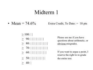
41. Supply Side (Closed) • Diminishing marginal productivity – as the amount of a certain input increases, holding all other inputs constant, the added benefit of each additional unit decreases Intuitive explanation – If you buy more computers without hiring more employees, you reach a point where there isn’t enough labour available to properly use all the capital

42. Production Function of L Y output L labour

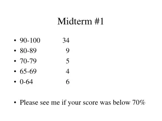
43. Labor supply equilibrium real wage MPL, Labor demand Supply Side (Closed) Labor supply MPL, Labor demand

44. Labor supply equilibrium rental MPL, Labor demand Supply Side (Closed) Supply of capital MPK, Demand for capital

45. Supply Side (Closed) • Conclusions: MPK = R/P = r MPL = W/P = w Expenditure on capital = MPK x K = rK Expenditure on labour = MPL x L = wL Total Expenditure = rK + wL = Y Expenditure = Output

46. Supply Side (Closed) • Alternatively, recall that α = share of income dedicated to capital MPK x K = rK = αY Y = rK/ α MPL x L = wL = (1 – α)Y Y = wL/(1 – α)

47. Supply Side (Closed) • Also recall that Y = A(Kα)(L(1- α)) A(Kα)(L(1- α)) = rK/ α (from previous slide) α A(Kα - 1)(L(1 - α)) = r = MPK A(Kα)(L(1- α)) =wL/(1 – α) (1 – α) A(Kα)(L(-α)) = w = MPL

48. Supply Side (Closed) • Key Formulas Y = A(Kα)(L(1- α)) Y = rK + wL MPK = r = R/P MPL = w = W/P

49. Supply Side (Closed) • Example: An economy has a nominal wage rate of $8 and a nominal rental rate of $6. The price level is 2. At these prices, the economy employ 5 units of labour and 3 units of capital. Calculate the MPK, MPL, and output.

50. Supply Side (Closed) Answer: MPK = R/P = 6/2 = 3 = r MPL = W/P = 8/2 = 4 = r Y = rK + wL Y = 3(3) + 4(5) Y = 29