Download
1 / 31
310 likes | 448 Views
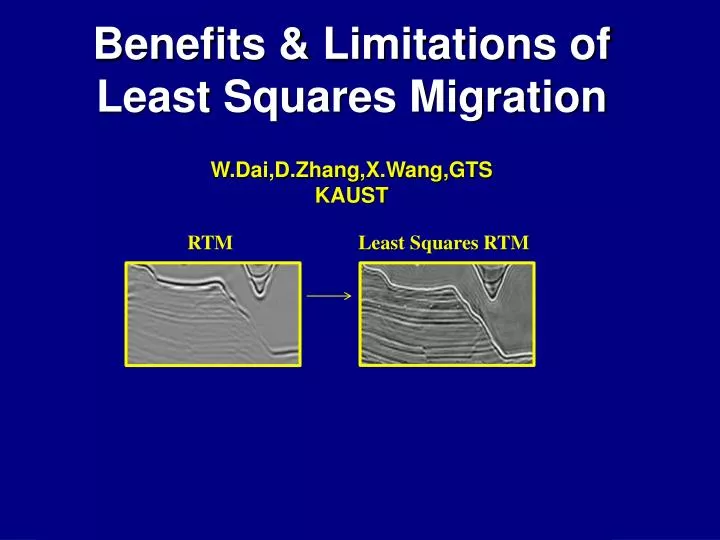
Benefits & Limitations of Least Squares Migration W.Dai,D.Zhang,X.Wang,GTS KAUST. RTM Least Squares RTM. GOM RTM GOM LSRTM. Can We Improve Quality Seismic Imaging?. Better Velocity Updates : FWI & MVA. Better Quality Images: LSM & Multiples.

E N D
Benefits & Limitations of Least Squares Migration W.Dai,D.Zhang,X.Wang,GTS KAUST RTM Least Squares RTM GOM RTM GOM LSRTM
Can We Improve Quality Seismic Imaging? Better Velocity Updates: FWI & MVA Better Quality Images: LSM & Multiples
Outline • Theory: Multisource LSM • Examples: Synthetic & Field Data • Summary
Standard Migration vs Multisource Migration Romero, Ghiglia, Ober, & Morton, Geophysics, (2000) Given: d1 and d2 Given: d1+ d2 Find: m Find: m Soln: m = (L1 + L2)(d1+d2) T T T Soln: m=L1 d1 + L2 d2 T T = L1 d1 + L2 d2 Benefit: Reduced computation and memory T T Liability: Crosstalk noise … + L1 d2 + L2 d1
Multisource LSM & FWI Inverse problem: 1 ~ ~ m || d – L m ||2 arg min J = 2 d misfit Iterative update: ~T m(k+1) = m(k) + aL d K=1 T T L1 d1 + L2 d2 K=10 T T + L1 d2 + L2 d1
Brief Early History Multisource Phase Encoded Imaging Migration Romero, Ghiglia, Ober, & Morton, Geophysics, (2000) Waveform Inversion and Least Squares Migration Krebs, Anderson, Hinkley, Neelamani, Lee, Baumstein, Lacasse, SEG Zhan+GTS, (2009) Virieux and Operto, EAGE, (2009) Dai, and GTS, SEG, (2009) Biondi, SEG, (2009)
Outline • Theory: Multisource LSM • Examples: 2D Marmousi Data • Summary
Migration Images (input SNR = 10dB) (Huang and Schuster, 2011, Multisource Least-squares Migration of Marine Streamer with Frequency-division Encoding ) SNR=30dB 304 shots in total an example shot and its aperture 0 0 b) Standard Migration a) Original Z (km) Z (km) Computational gain 1.48 1.48 9.4 8.0 6.6 5.4 6.75 X (km) 0 • d) 304 shots/gather • 26 iterations c) Standard Migration with 1/8 subsampled shots Conventional migration: 1 Comp. Gain Shots per supergather 76 152 304 38 6.75 6.75 X (km) X (km) 0 0
Sensitivity to input noise level 9.4 8.0 SNR=30dB 6.6 5.4 SNR=10dB 3.8 Computational gain SNR=20dB Conventional migration: 1 38 76 152 304 Shots per supergather
Outline • Theory: Multisource LSM • Examples: 3D SEG Salt • Summary
SEG/EAGE Model+MarineData (Yunsong Huang) • sources in total 40m 100 m 16 swaths, 50% overlap 256 sources a swath 6 km 20 m 3.7 km 16 cables 13.4 km
Numerical Results (Yunsong Huang) True reflectivities Conventional migration 6.7 km 3.7 km 256shots/super-gather,16iterations 3.7 km 13.4 km 8 x gain in computational efficiency
Outline • Theory: Multisource LSM • Examples: 2D GOM Data LSRTM • Summary
Plane-wave LSRTM of 2D GOM Data • Model size: 16 x 2.5 km. • Source freq: 25 hz • Shots: 515 • Cable: 6km • Receivers: 480 km/s 0 2.1 Z (km) 2.5 1.5 16 0 X (km)
Conventional GOM RTM (cost: 1) (Wei Dai) Plane-wave LSRTM (cost: 12) 0 Z (km) 2.5 Encoded Plane-wave LSRTM (cost: 0.4) Plane-wave RTM (cost: 0.2) 0 Z (km) 2.5 16 0 X (km)
Conventional GOM RTM (cost: 1) (Wei Dai) Plane-wave LSRTM (cost: 12) 0 Z (km) LSM RTM 2.5 Encoded Plane-wave LSRTM (cost: 0.4) Plane-wave RTM (cost: 0.2) 0 Z (km) 2.5 16 0 X (km)
Outline • Theory: Multisource LSM • Examples: 2D GOM Data KLSM • Summary • Theory: Multisource LSM • Examples: 2D GOM Data LSRTM • Summary
Kirchhoff Migration Image (1X) 1.5 Z (km) 0.9 K M Multisource Least-squares Migration Image (>10X) 1.5 Z (km) 0.9 KLS M (X. Wang) 10.5 X (km) 11.5
Alias and Gap Data GOM data, aliased source and gap between 9.5 km and 10 km Velocity model 2.5 Z (km) 0 Model Size: 3407 X 401 km/s 2.2 Interval: 6.25 m # of shots: 248, ds = 75 m # of receiver: 480, dg = 12.5 m Streamer length: 6 km Record length: 10.24 s, dt=2ms 0 X(km) 18.8 1.5 # of supergather: 32 # of shots in supergather: 16 Velocity model is from FWI. (Boonyasiriwat et al., 2010) A 10-15-70-75 Hz bandpass filter is applied. Source wave is generated from stacking near offset ocean bottom reflections.
Plane-wave LSRTM of 2D GOM Data • Model size: 16 x 2.5 km. • Source freq: 25 hz • Shots: 515 • Cable: 6km • Receivers: 480 km/s Mute 0.5 km data 0 2.1 Z (km) 2.5 1.5 16 0 X (km)
KM VS LSM VS MSLSM KM image
KM VS LSM VS MSLSM LSM Image after 30 Iterations
KM VS LSM VS MSLSM MSLSM Image after 30 Iterations
Outline • Theory: Multisource LSM • Examples: 2D Salt Body with Multiples • Summary
RTM SEG Salt Data (Dongliang Zhang) 0 Z (km) 16 LSRTM with Born Multiples 0 1st-order Multiples Z (km) 16 0 X (km) 16
RTM SEG Salt Data (Dongliang Zhang) 0 Z (km) 16 LSRTM with Born Multiples 0 RTM LSRTM Z (km) 16 0 X (km) 16
GOM Salt Data (Dongliang Zhang) 0 Z (km) 3.0 RTM with Multiples 0 Z (km) 3.0 0 X (km) 30
Starting Velocity Model 0 Z (km) 3.0 FWI (Abdullah AlTheyab) 0 Z (km) 3.0 0 X (km) 30
What have we Empirically Learned about Quality? • LSM no better than RTM if inaccurate v(x,y,z) 2. Cost MLSM ~ RTM; MLSM better resolution 3. Speckle noise in LSM 4. Multiples can be significantly enhanced if separated properly from primaries 5. FWI works for easy GOM data, not for hard salt 6. FWI & LSM quality degrades below 2 km? 7. Why? Unaccounted Physics? 1). Attenuation, 2). V(x,y,z), 3). ???
True Reflectivity Q Model 0 Z (km) 1.5 0 Z (km) 1.5 Q=20000 Q=20 0 X (km) 2 0 X (km) 2 Acoustic LSRTM Viscoelastic LSRTM 0 Z (km) 1.5 1.0 -1.0 1.0 -1.0 0 X (km) 2 0 X (km) 2
What have we empirically learned about MLSM? Stnd. MigMultsrc. LSM IO 1 ~1/36 1 ~0.1 Cost Migration SNR ~1 1 Resolution dx1 ~double Cost vs Quality: Can I<<S? Yes.