2.4 Audio Compression

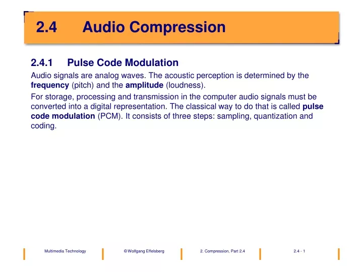
1. 2.4 Audio Compression • 2.4.1 Pulse Code Modulation • Audio signals are analog waves. The acoustic perception is determined by the frequency (pitch) and the amplitude (loudness). • For storage, processing and transmission in the computer audio signals must be converted into a digital representation. The classical way to do that is called pulsecode modulation (PCM). It consists of three steps: sampling, quantization and coding.

2. Sampling • The analog signal is sampled periodically. At each sampling interval the analog value of the signal (e.g., the voltage level) is recorded as a real number. • After sampling the signal is no longer continuous but discrete in the temporal dimen-sion.

3. Sampling Theorem of Nyquist • In order to reconstruct the original analog signal without loss we obviously need a minimum sampling frequency. The minimum sampling frequency fA is given by the sampling theorem of Nyquist (1924): • For noise-free channels the sampling frequency fA must be twice as high as the highest frequency occurring in the signal: • fA = 2 fS

4. Example: Sampling a Signal at Different Rates

5. Quantization • The range of values occurring in the analog signal is subdivided into a fixed number of discrete intervals. Since all analog values contained in an interval will be mapped to the same interval number (corresponding to the middle of the interval) we intro-duce a quantization error. If the size of the quantization interval is a then the maxi-mum quantization error is a/2.

6. Binary Coding • We now have to determine a unique binary representation for each quantization inter-val. In principle any binary code does the job. The simplest code (which is in fact often used in practice) is to encode each interval with a fixed-size binary number.

7. PCM: The Complete Process • The combination of the steps sampling, quantization and binary coding is called Pulse Code Modulation (PCM).

8. CODECs • The devices performing A/D conversion and D/A conversion are called CODECs (Coders/Decoders). Note: A modem is used to transmit digital signals over analog links, a codec is used to transmit analog signals over digital links.

9. PCM Telephone Channel • Sampling Rate • Starting point: an analog ITU-T telephone channel • Frequency range: 300 – 3400 Hz, i.e., audiobandwidth: 3100 Hz (sufficient for speech) • Sampling frequency: fA = 8 kHz • Sampling period: TA = 1/ fA = 1/8000 Hz = 125 μs • The sampling frequency chosen by ITU-T is higher than the Nyquist limit: for a maximum frequency of 3400 Hz in the signal a sampling frequency of 6800 Hz would be sufficient. The higher sampling frequency has technical reasons (noise, influence of filters, channel separation, etc.)

10. Quantization of the Amplitude • The minimum number of quantization intervals is determined by the understandability of speech at the receiver. Based on experimental experience ITU-T has chosen 256 quantization intervals. • With standard binary coding we thus need 8 bits per sample. • Bit Rate of the PCM Channel • We conclude that the bit rate of a standard PCM channel is 8 bits * 8000/s = 64 kbit/s.

11. Non-Linear Quantization • With linear quantization all intervals have the same size, they do not depend on the amplitude of the signal. However it would be desirable to have a smaller amount of quantization noise at small amplitude levels because quantization noise is more disturbing in “quiet times“. • This goal can be reached with non-linear quantization. We simply chose larger quantization intervals at higher amplitude values. • Technically this can be done by a “signal compressor“ which precedes the coding step. At the receiver side an expander is used to reconstruct the original dynamics. • Many compressors use a logarithmic mapping. In digital electronics this is often approximated by a piecewise-linear curve. The 13-segment compressor curve is a typical example.

12. 13-Segment Compressor Curve

13. Delta Modulation • Instead of coding the absolute values of the amplitude, the difference to the value in the previous interval is coded in one bit. Only steps of +1 or –1 are possible. Coding: 1 = increasing signal 0 = decreasing signal

14. Differential PCM (DPCM) • In differential PCM we encode the actual difference between the signal values in two adjacent intervals with a small number of bits. This leads to a bit rate and precision between that of encoding the absolute values and delta modulation. • Adaptive DPCM (ADPCM) • The dynamics in real audio signals are often such that we have quiet periods and loud periods. In quiet periods (i.e., periods with low variance of the amplitude) we can encode the signal with fewer bits than in loud periods. This is called Adaptive Pulse Code Modulation (ADPCM). • For example, ADPCM allows us to compress a HiFi stereo audio signal from 1.4 Mbit/s to 0.2 Mbit/s without loss of quality. • Well-known ADPCM algorithms are μ-law and A-law.

15. Typical Sampling and Quantization Parameters • Sampling Rate • 8 kHz telephony, μ-law encoding, SUN audio • 32 kHz Digital Radio Broadcast • 44,1 kHz Audio CD • 48 kHz Digital Audio Tape (DAT) • Quantization • 8 bits 256 amplitude levels: speech • 16 bits 65536 amplitude levels: HiFi music

16. 2.4.2 Audio Compression with Psycho-Acoustic Models • Compression Based on Semantic Relevance • We remove those parts of the signal at the source that the receiver will not be able to hear anyway. • Example: The Masking Effect • A high-amplitude signal masks out a low-amplitude signal at an adjacent frequency.

17. Psycho-Acoustic Models

18. Example: MPEG Audio • Characteristics • Compression to 32, 64, 96, 128 or 192 kbit/s • Audio channels • mono or • two independent channels or • “joint stereo" • Techniques • Sampling rates: 32 kHz, 44,1 kHz or 48 kHz • 16 bits per sample • Maximum encoding and decoding delay: 80 ms at 128 kbit/s • A psycho-acoustic model controls the quantization.

19. Two Techniques in MPEG-1 Audio

20. MPEG Audio Encoder and Decoder • Encoder Decoder

21. Three Layers in MPEG Audio • Sub-band coding with 32 bands with the MUSICAM technique • high data rate • mono, stereo, 48 kHz, 44.1 kHz, 32 kHz • Sub-band coding with MUSICAM, more complex psycho-acoustic model • intermediate • better sound quality at low bit rates • Transformation-based compression with the ASPEC technique • lowest data rate • stereo audio in CD quality at less than 128 kbit/s! • mono audio in telephone quality at 8 kbit/s • MPEG audio layer 3, encoded with ASPEC, is also called MP3!

22. MP3 – History (1) • As early as 1987 the Fraunhofer Institut für Integrierte Schaltkreise (Institute of Integrated Circuits) in Erlangen (Germany) began with the development of audio compression techniques that took the specific properties of the human perceptual system into account. Their technique was included into the MPEG Audio standard of ISO (IS-11172-3 and IS 13818-3) as MPEG Audio Layer 3 (MP3). • The original goal was a reduction of the data rate by a factor of 12 compared to an audio CD, with no audible difference.

23. MP3 – History (2) • As usual, ISO only standardizes the technical parameters and the decoder. The inner workings of the encoder remain unspecified. This gives developers significant freedom to develop specific encoding techniques, and even get patents for their encoding algo-rithms. • As a consequence we know very little about the exact implementation of the MP3 en-coder written by the Fraunhofer Institute. Exact details on their psycho-acoustic model are not published. The Fraunhofer Institute also holds a patent on its optimized enco-ding mechanism for MP3.

24. MPEG Audio Encoding (1) • MP3 subdivides the data stream into frames. Each frame corresponds to the audio signal in a certain time period. It contains 384 samples. The samples represent values out of 32 frequency sub-bands. There are 12 values from each sub-band.

25. MPEG Audio Encoding (2) • Step 1 • Frequency masking: Usage of a DCT-based filter. At any given time the algorithm only considers one frame. The frequencies occurring in this frame are subdivided into the frequency bands and then filtered. • Step 2 • Temporal masking: At any given time the algorithm looks at three adjacent frames, the previous, the current and the next frame. This allows to take advantage of tem-poral masking effects as perceived by the human ear. • Step 3 • Non-linear masking: The frequencies are subdivided into bands of different widths. Also, stereo channels are encoded differentially, i.e., the difference between the two channels rather than the absolute values are encoded. The last step is a Huffman coding of the coefficients.

26. Step 1: Psycho-Acoustic Effect • 1. Sensitivity of the human ear 2. The frequency masking effect Experiment: Play a tone of 1 kHz (the masking tone) at a certain amplitude (e.g., 60 dB). Then add a test tone (e.g., of 1.1 kHz) and increase its amplitude until the the test tone is heard. This will happen at a much higher amplitude than in the quiet.

27. Step 1: Compression • Apply a sub-band filter to subdivide the signal into 32 bands (“critical bands“). For each band, define a masking curve that indicates at which level the signal will be masked by adjacent bands. • Algorithm • Compute the energy in each band. • If the energy in a band is smaller than the masking threshold of a neighboring band, do not encode the band. • Otherwise encode the band. Quantize the coefficients with a quantization factor. Choose the factor so that the quantization error is smaller than the masking factor (one bit in the quantization corresponds to a noise of 6 dB).

28. Step 1: Example • The table shows the levels of the first 16 out of the 32 bands. • ---------------------------------------------------------------------------------------------- • Band 1 2 3 4 5 6 7 8 9 10 11 12 13 14 15 16 • Level 0 8 12 10 6 2 10 60 35 20 15 2 3 5 3 1 • ---------------------------------------------------------------------------------------------- • The level of band 8 is 60 dB. We assume that it has a masking threshold of 12 dB for band 7 and of 15 dB for band 9. • The level of band 7 is 10 dB (< 12 dB), thus we ignore it. • The level of band 9 is 35 dB (> 15 dB), thus we encode it. We choose the quantization factor so that the quantization error will be less than 2 bits (12 dB).

29. Step 2: Psycho-Acoustic Effect • Temporal masking: When we hear a loud sound that suddenly stops it takes a while until we can hear soft sounds again. • Experiment: Play a masking tone of 1 kHz at 60 dB and a 1.1 kHz test tone at 40 dB (the test tone is not heard, it is masked). Stop the masking tone and after a short de-lay also the test tone. Vary the delay to find the time threshold at which the test tone can just be heard.

30. Step 2: Compression • Repeat the experiment with other test tones: In a way similar to step 1, we take advantage of this temporal phenomenon to mask out sub-bands, this time those of adjacent frames. For simplification we assume that a sub-band can mask out its neighbors only in one preceding and one succeeding frame.

31. Step 3: Psycho-Acoustic Effect • The contrast resolution of the human ear decreases with the frequency of the signal. • In layers 1 and 2 the frequency spectrum is subdivided into 32 critical bands of ident-ical size. In layer 3, the frequencies are distributed in a non-linear fashion, in a way so that all bands contribute equally to the perception by the ear.

32. Step 3: Compression • Masking Thresholds on critical band scale: Step 3 comes closer to human perception by choosing a more appropriate defi-nition of the sub-bands. In addition to frequency masking and temporal masking, as in layers 1 and 2, layer 3 also introduces the differential coding of stereo signals, as well as an entropy en-coding of the coefficients based on the Huffman code.

33. Performance of MP3 • Quality measure: • 5 = perfect, 4 = just noticeable, 3 = slightly annoying, 2 = annoying, 1 = very annoying • The real delay is about three times the theoretical minimum delay.

34. 2.4.3 Speech Coding • Special codecs optimized for the human voice can reach a very high speech quality at very low data rates.They operate at the normal range of the voice, i.e., at 300 - 3400 Hz. • Such special codecs are most often based on Linear Predictive Coding (LPC).

35. Linear Predictive Coding (1) • LPC models the anatomy of the human voice organs as a system of connected tubes of different diameters.

36. Linear Predictive Coding (2) • Acoustic waves are produced by the vocal cords, flow through a system of tubes, are partially reflected at the transitions and interfere with the following waves. • The reflection rate at each transition is modeled by the reflection coefficient refl[0], ..., refl[p-1]. • We can thus characterize the (speaker-dependent) production of the voice signal with a very small number of parameters.

37. LPC Encoder (1) • The LPC Algorithm • The audio signal is decomposed into small frames of fixed length (20 – 30 ms). For each frame s[i] we compute p weights lpc[0], .. , lpc[p-1] so that s[i] is approximated bylpc[0] * s[i-1] + lpc[1] * s[i-2] + ... + lpc[p-1] * s[i-p] • Popular values for p are 8 or 14. • A synthetically generated source signal is used as input to the model. The gene-rated source can be switched between two modes: voiced (for vowels) and noise (voiceless, for consonants). • The differences between the synthetically generated signal and the real voice sig-nal during the frame are detected and used to re-calculate the prediction coeffi-cients lpc[i]. • For each frame the mode of excitation (voiced or voiceless) and the current values of the parameters are encoded and transmitted.

38. LPC Encoder (2) • The LPC Algorithm Synthesized or stored part of the wave Predicted part of the wave Usually the number of constraints (rows) is much larger than the number of coefficients (columns). The optimization aims at choosing the coefficients such that the errors ei are minimized.

39. LPC Variations • CELP (Code Excited Linear Prediction): We not only distinguish “voiced“ and “voiceless“ but many more types of excitation. These are pre-defined by the developers and stored in the form of a “codebook“. For each frame we transmit the index into the codebook and the lpc parameters. • ACELP: like CELP, but with an adaptive codebook

40. LPC Examples • G.723.1 • Adaptive CELP Encoder (Code Excited Linear Predictor). • Bit rate for G.723.1: 5,3 kbit/s - 6.3 kbit/s • GSM 06.10 • Regular Pulse Excitation – Long Term Prediction (RPE-LTP) • LPC encoding • Bit rate for GSM 06.10: 13.2 kbit/s

41. Specialized Speech Coding vs. PCM Coding

42. ITU-T Standards for Speech Coding • A selection from the G.7xx-Standards • G.711: 64 kbit/s (PSTN telephony, H.323 and H.320 videoconferencing) • G.728 LD-CELP: 16 kbit/s (GSM telephony, H.320 videoconferencing) • G.729 ACELP: 8 kbit/s (GSM telephony, H.324 video telephony) • G.723.1 MPE/ACELP 5.3 kbit/s up to 6.3 kbit/s (GSTN video telephony, H.323 telephony)