Download
1 / 15
160 likes | 581 Views
Multiple Regression. More than one explanatory/independent variable This makes a slight change to the interpretation of the coefficients This changes the measure of degrees of freedom We need to modify one of the assumptions EXAMPLE: tr t = 1 + 2 p t + 3 a t + e

E N D
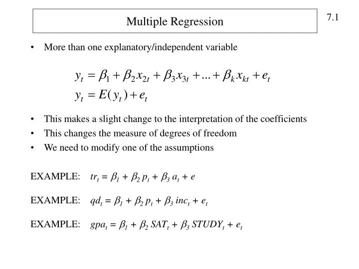
Multiple Regression • More than one explanatory/independent variable • This makes a slight change to the interpretation of the coefficients • This changes the measure of degrees of freedom • We need to modify one of the assumptions EXAMPLE: trt = 1 + 2 pt + 3 at + e EXAMPLE: qdt = 1 + 2 pt + 3 inct + et EXAMPLE: gpat = 1 + 2 SATt + 3 STUDYt + et
Interpretation of Coefficient • 2 measures the change in Y from a change in X2, holding X3 constant. • 23 measures the change in Y from a change in X3, holding X2 constant.
Assumptions of the Multiple Regression Model • The Regression Model is linear in the parameters and error term yt = 1 + 2 x2t + 3 x3t + … k xkt +et 2. Error Term has a mean of zero: E(e) = 0 E(y) = 1 + 2 x2t + 3 x3t + … k xkt 3. Error term has constant variance: Var(e) = E(e2) = 2 4. Error term is not correlated with itself (no serial correlation): Cov(ei,ej) = E(eiej) = 0 ij • Data on x’s are not random (and thus are uncorrelated with the error term: Cov(X,e) = E(Xe) = 0) and they are NOT exact linear functions of other explanatory variables. • (Optional) Error term has a normal distribution. E~N(0, 2)
Estimation of the Multiple Regression Model • Let’s use a model with 2 independent variables: • A scatterplot of points is now a scatter “cloud”. We want to fit the best “line” through these points. In 3 dimensions, the line becomes a plane. • The estimated “line” and a residual are defined as before: • The idea is to choose values for b1, b2, and b3 such that the sum of squared residuals is minimized.
From here, we minimize this expression with respect to b1, b2, and b3. We set these three derivatives equal to zero and Solve for b1, b2, b3. We get the following formulas: Where:
[What is going on here? In the formula for b2, notice that if x3 where omitted from the model, the formula reduces to the familiar formula from Chapter 3.] You may wonder why the multiple regression formulas on slide 7.5 aren’t equal to:
We can use a Venn diagram to illustrate the idea of Regression as Analysis of Variance For Bivariate (Simple) Regression y x For Multiple Regression y x2 x3
Example of Multiple Regression Suppose we want to estimate a model of home prices using data on the size of the house (sqft), the number of bedrooms (bed) and the number of bathrooms (bath). We get the following results: How does a negative coefficient estimate on bed and bath make sense?
Variance Formulas With 2 Independent Variables Expected Value We will omit the proofs. The Least Squares estimator for multiple regression is unbiased, regardless of the number of independent variables Where r23 is the correlation between x2 and x3 and the parameter 2 is the variance of the error term. We need to estimate 2 using the formula This estimate has T-k degrees of freedom.
Gauss Markov Theorem Under the assumptions 1-5 (the 6th assumption isn’t needed for the theorem to be true) of the linear regression model, the least squares estimators b1, b2, …bk have the smallest variance of all linear and unbiased estimators of 1 , 2,… k. They are the BLUE (Best, linear, unbiased, estimator)
Confidence Intervals and Hypothesis Testing • The methods for constructing confidence intervals and conducting hypothesis tests are the same as they were for simple regression. • The format for a confidence interval is: Where tc depends on the level of confidence and has T-k degrees of freedom. T is the number of observations and k is the number of independent variables plus one for the intercept. • Hypothesis Tests: Ho: i = c H1: i c Use the value of c for i when calculating t. If t > tc or t < - tc reject Ho If c is 0, then we call it a test of significance.
Goodness of Fit • R2 measures the proportion of the variance in the dependent variable that is explained by the independent variable. Recall that • Least Squares chooses the line that produces the smallest sum of squared residuals, it also produces the line with the largest R2. It also has the property that the inclusion of additional independent variables will never increase and will often lower the sum of squared residuals, meaning that R2 will never fall and will often increase when new independent variables are added, even if the variables have no economic justification. • Adjusted R2: adjust R2 for degrees of freedom
Example: Grades at JMU • A sample of 55 JMU students was taken Fall 2002. Data on • GPA • SAT scores • Credit Hours Completed • Hours of Study per Week • Hours at a Job per week • Hours at Extracurricular Activites Three models were estimated: gpat = 1 + 2 SATt + et gpat = 1 + 2 SATt + 3 CREDITSt + 4 STUDYt + 5JOBt + 6 ECt + et gpat = 1 + 2 SATt + 3 CREDITSt + 4 STUDYt + 5JOBt + et
Here is our simple Regression model. Here is our multiple regression model. Both R2 and Adjusted R2 have increased with the inclusion of 4 additional indep. variables.
Notice that the Exclusion of EC increases adjusted R2 but reduces R2