Download
1 / 37
370 likes | 654 Views
Similarity in CBR. Sources: Chapter 4 www.iiia.csic.es/People/enric/AICom.html www.ai-cbr.org. similarity. similarity. Computing Similarity. Similarity is a key (the key?) concept in CBR. We saw that a case consists of:. Problem Solution Adequacy.

E N D
Similarity in CBR Sources: Chapter 4 www.iiia.csic.es/People/enric/AICom.html www.ai-cbr.org
similarity similarity Computing Similarity • Similarity is a key (the key?) concept in CBR • We saw that a case consists of: • Problem • Solution • Adequacy • We saw that the CBR problem solving cycle consists of: • Retrieval • Reuse • Revise • Retain • We will distinguish between: • Meaning of similarity • Formal axioms capturing this meaning
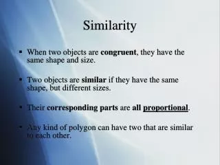
Meaning of Similarity • Observation 1: Similarity always concentrates on one aspect or task: • There is no absolute similarity • Example: • Two cars are similar if they have similar capacity (two compact cars may be similar to each other but not to a full-size car) • Two cars are similar if they have similar price (a new compact car may be similar to an old full-size car but not to an old compact car) • When computing similarity we are concentrating on one such aspect or aggregating several such aspects
Meaning of Similarity (2) • Observation 2: Similarity is not always transitive: • Example: • I define similar to mean “within walking distance” • “Lehigh’s book store” is similar to “Lupita” • “Lupitas” is similar to “Perkins” • “Perkins” is similar to “Monrovia book store” • … • But: “Lehigh’s book store” is not similar to “Best Buy” in Allentown ! • The problem is that the property “small difference” cannot be propagated
Meaning of Similarity (3) • Observation 3: Similarity is not always symmetric: • Example: • “Mike Tyson fights like a lion” • But do we really want to say that “a lion fights like Mike Tyson”? • The problem is that in general the distance from an element to a prototype of a category is larger than the other way around
Similarity and Utility in CBR • Utility: measure of the improvement in efficiency as a result of a body of knowledge (We’ll come back to this point) • The goal of the similarity is to select cases that can be easily adapted to solve a new problem Similarity = Prediction of the utility of the case • However: • The similarity is an a priori criterion • The utility is an a posteriori criterion • Ideal: Similarity makes a good prediction of the utility
Axioms for Similarity • There are 3 types of axioms: • Binary similarity predicate “x and y are similar” • Binary dissimilarity predicate “x and y are dissimilar” • Similarity as order relation: “x is at least as similar to y as it is to z” • Observation: • The first and the second are equivalent • The third provides more information: grade of similarity
Similarity Relations • We want to define a relation: • R(x,y,z) iff “x is at least as similar to y as x is similar is to z” • First lets consider the following relation: • S(x,y,u,v) iff “x is at least as similar to y as u is similar to v” • Definition of R in terms of S: R(x,y,z) iff S(x,y,x,z)
Similarity Relations (2) • Possible requirements on the relation S: • Reflexive: S(x,x,u,v) • Symmetry: S(x,y,y,x) • Transitivity: S(x,y,u,v) & S(u,v,s,t) S(x,y,s,t) • Symmetry: S(x,y,u,v) iff S(y,x,u,v) iff S (x,y,v,u)
Similarity Relations (3) • In CBR we have an object x fixed when computing similarity. Which x? The new problem • We are looking for a y such that y is the most similar to x. In terms of R this be seen as: z: R(x,y,z) • Given a problem x we can define an ordering relation x as follows: • y x z iff R(x,y,z) • y >x z iff (y x z and ¬ z x y) • y ~x z iff (y x z and z x y)
Similarity Metric • We want to assign a number to indicate the similarity between a case and a problem • Definition: A similarity metric over a set M is a function: • sim: M M [0,1] • Such that: • For all x in M: sim(x,x) = 1 holds • For all x, y in M: sim(x,y) = sim(y,x) “ the closer the value of sim(x,y) to 1, the more similar is x to y”
sim provides a quantitative value for similarity: sim(x, yi) y1 y2 y3 y4 0 1 Thus y4 is more similar to x Similarity Metric (2) • Given a similarity metric: sim: M M [0,1], it induces a similarity relation Ssim (x,y,u,v) and xas follows: • For all x, y, u, v: Ssim(x,y,u,v) holds if • For all x, y, z: y x z if sim(x,y) sim(u,v) sim(x,y) sim(x,z)
Distance Metric • Definition: A distance function over a set M is a function: • d: M M [0,) • Such that: • For all x in M: d(x,x) = 0 holds • For all x, y in M: d(x,y) = d(y,x) • Definition: A distance function over a set M is a metric if: • For all x, y in M: d(x,y) = 0 holds then x = y • For all x, y, z in M: d(x,z) + d(z,y) d(x,y)
Relation between Similarity and Distance Metric • Given a distance metric, d, it induces a similarity relation Sd(x,y,u,v), xas follows: • For all x, y, u, v: S(x,y,u,v) holds if • For all x, y, z: y x z if d(x,y) d(u,v) d(x,y) d(x,z) Definition: A similarity metric sim and a distance metric d are compatible iff: for all x,y, u, v: Sd(x,y,u,v) iff Ssim(x,y,u,v)
f(d(x,y)) > f(d(u,v)) Relation between Similarity and Distance Metric (2) • Property: Let • f: [0,) (0,1] • Be a bijective and order inverting (if u< v then f(v) < f(u)) function such that: • f(0) = 1 • f(d(x,y)) = sim(x,y) • then d and sim are compatible If d(x,y) < d(u,v) then sim(x,y) > sim(u,v)
Relation between Similarity and Distance Metric (3) • F(x) can be used to construct sim giving d. Example of such a function is: • if you have the Euclidean distance: • d((x,y),(u,v)) = sqr((x-u)2 + (y-v)2) • Since f(x) = 1 – (x/(x+1)) meets the property before • Then: • sim((x,y),(u,v))) = f(d((x,y),(u,v))) • = 1 – (d((x,y),(u,v)) /(d((x,y),(u,v)) +1)) • is a similarity metric
Relation between Similarity and Distance Metric (3) • The function f(x) = 1 – (x/(x+1)) is a bijective function from [0,) into (0,1]: 1 0
Other Similarity Metrics • Suppose that we have cases represented as attribute-value pairs (e.g., the restaurant domain) • Suppose initially that the values are binary • We want to define similarity between two cases of the form: • X = (X1, …, Xn) where Xi = 0 or 1 • Y = (Y1, …,Yn) where Yi = 0 or 1
Preliminaries • Let: • A = (i=1,n)Xi•Yi • B = (i=1,n)Xi•(1-Yi) • C = (i=1,n)(1-Xi)•Yi • D = (i=1,n)(1-Xi) •(1-Yi) • Then, A + B + C + D = (number of attributes for which Xi =1 and Yi = 1) (number of attributes for which Xi =1 and Yi = 0) (number of attributes for which Xi =0 and Yi = 1) (number of attributes for which Xi =0 and Yi = 0) n “matching attributes” “mismatching attributes” A+D = B+C=
Hamming Distance H(X,Y) = n –(i=1,n)Xi•Yi–(i=1,n)(1-Xi)•(1-Yi) • Properties: • Range of H: • H counts the mismatch between the attribute values • H is a distance metric: • H((1-X1, …, 1-Xn), (1-Y1, …,1-Yn)) = [0,n] • H(X,X) = 0 • H(X,Y) = H(Y,X) H((X1, …, Xn), (Y1, …,Yn))
Proportion of the difference # of mismatches Simple-Matching-Coefficient (SMC) n – (A + D) = B + C • H(X,Y) = • Another distance-similarity compatible function is • f(x) = 1 – x/max (where max is the maximum value for x) • We can define the SMC similarity, simH: simH(X,Y) = 1 – ((n – (A+D))/n) = (A+D)/n = 1- ((B+C)/n)
Simple-Matching-Coefficient (SMC) (II) • If we use on simH(X,Y) = (A+D)/n =1- ((B+C)/n) = factor(A, B, C, D) • Monotonic: • If A A’ then: • If B B’ then: • If C C’ then: • If D D’ then: factor(A,B,C,D) factor(A’,B,C,D) factor(A,B’,C,D) factor(A,B,C,D) factor(A,B,C’,D) factor(A,B,C,D) factor(A,B,C,D) factor(A,B,C,D’) • Symmetric: • simH (X,Y) = simH(Y,X)
Variations of the SMC • The hamming similarity assign equal value to matches (both 0 or both 1) • There are situations in which you want to count different when both match with 1 as when both match with 0 • Thus, sim((1-X1, …, 1-Xn), (1-Y1, …,1-Yn)) = sim((X1, …, Xn), (Y1, …,Yn)) may not hold • Example: Two symptoms of patients are similar if they both have fever (Xi = 1 and Yi = 1) but not similar if neither have fever (Xi = 0 and Yi = 0) • Specific attributes may be more important than other attributes Example: manufacturing domain: some parts of the workpiece are more important than others
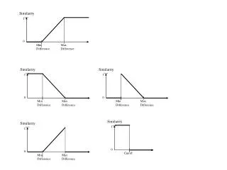
Variations of SMC (III) • simH(X,Y) = (A+D)/n = (A+D)/(A+B+C+D) • We introduce a weight, , with 0 < < 1: sim(X,Y) = ((A+D))/ ((A+D) + (1 - )(B+C)) • For which is sim(X,Y) = simH(X,Y)? = 0.5 • sim(X,Y) preserves the monotonic and symmetric conditions
1 > 0.5 = 0.5 < 0.5 0 n 0 The similarity depends only from A, B, C and D (3) • What is the role of ? What happens if > 0.5? If < 0.5? sim(X,Y) = ((A+D))/ ((A+D) + (1 - )(B+C)) • If > 0.5 we give more weights to the matching attributes • If < 0.5 we give more weights to the miss-matching attributes
Discarding 0-match • Thus, sim((1-X1, …, 1-Xn), (1-Y1, …,1-Yn)) = sim((X1, …, Xn), (Y1, …,Yn)) may not hold • Only when the attribute occurs (i.e., Xi = 1 and Yi = 1 ) will contribute to the similarity • Possible definition of the similarity: sim = A / (A+ B+C)
Specific Attributes may be More Important Than Other Attributes • Significance of the attributes varies • Weighted Hamming distance: • There is a weight vector: (1, …, n) such that • (i=1,n) i = 1 HW(X,Y) = 1 –(i=1,n) i • Xi•Yi–(i=1,n) i • (1-Xi)•(1-Yi) • Example: “Process planning: some features are more important than others”
Non Monotonic Similarity • The monotony condition in similarity, formally, says that: sim(A,B) sim(A’,B) • always holds if A counts the number of matches and A A’ • Informally the monotony condition can be expressed as: • For any X, Y, X’ attribute-value vectors, If we obtain X’ by modifying X on the value of one attribute such that X’ and Y have the same value on that attribute then: sim(X,Y) sim(X’,Y)
Non Monotonic Similarity (2) • Is the hamming distance monotonic? Yes simH(X,Y) = (i=1,n)eq(Xi,Yi) / n • Consider the XOR function: • (0,0) and (1,1) are on the same class (+) • (0,1) and (1,0) are on the same class (-) • Thus d((1,1),(1,0)) > d((1,1),(0,0)) • Is this monotonic? No
Suppose that we have two interconnected batteries B and B’ and 3 lamps X, Y and Z that have the following properties: • If X is on, B and B’ work • If Y is on, B or B’ work • If Z is on, B works Situation X Y Z B B’ • 0 1 1 Ok Fail • 0 1 0 Fail Ok • 0 0 0 Fail Fail Non Monotonic Similarity (3) • You may think: “well that was mathematics, how about real world?” • Thus: • sim(1,3) > sim(1,2) • Non monotonic!
P S A B C Tversky Contrast Model • Defines a non monotonic distance • Comparison of a situation S with a prototype P (i.e, a case) • S and P are sets of features • The following sets: • A = S P • B = P – S • C = S – P
Tversky Contrast Model (2) • Tversky-distance: • Where f: [0, ) • f, , , and are fixed and defined by the user • Example: • If f(A) = # elements in A • = = = 1 • T counts the number of elements in common minus the differences • The Tversky-distance is not symmetric T(P,S) = f(A) - f(B) - f(C)
Local versus Global Similarity Metrics • In many situations we have similarity metrics between attributes of the same type (called local similarity metrics). Example: For a complex engine, we may have a similarity for the temperature of the engine • In such situations a reasonable approach to define a global similarity sim(x,y) is to “aggregate” the local similarity metrics simi(xi,yi). A widely used practice • What requirements should we give to sim(x,y) in terms of the use of simi(xi,yi)? sim(x,y) to increate monotonically with each simi(xi,yi).
Local versus Global Similarity Metrics (Formal Definitions) • A local similarity metric on an attribute Ti is a similarity metric simi: Ti Ti [0,1] • A function : [0,1]n [0,1] is an aggregation function if: • (0,0,…,0) = 0 • is monotonic non-decreasing on every argument • Given a collection of n similarity metrics sim1, …, simn, for attributes taken values from Ti, a global similarity metric, is a similarity metric sim:V V [0,1], V in T1 … Tn, such that there is an aggregation function with: • sim(X,Y) = sim(X,Y) = (sim1(X1,Y1), …,simn(Xn,Yn)) Example: (X1,X2,…,Xn) = (X1+X2+…+Xn)/n
Example • Cases may contain attributes of type: • real number A: the voltage output of a device • define a local similarity metric, simvoltage() • Integer B: revolutions per second • define a local similarity metric, simrps() • A bunch of symbolic attributes m = (C1,..,Cm): front light blinking or none, year of manufacture, etc • define a Hamming similarity, simH(), combining all these attributes • Define an aggregated similarity sim() metric: sim(C,C’) = 1 *simvoltage(A,A’) + 2 *simvoltage(A,A’) + 3*simH(m, m’)
Homework (1 of 2) • In Slide 12 we define the similarity relation Ssim(x,y,u,v). Which of the 4 kinds of relations defined in Slide 9 are satisfied by Ssim(x,y,u,v)? • Let us define: SH(x,y,u,v) iff H(x,y) H(u,v) where H is the Hamming distance (defined in Slide 20). Which of the 4 kinds of relations defined in Slide 9 are satisfied by SH(x,y,u,v)? 3. Let us define: ST(x,y,u,v) iffT(x,y) T(u,v) where T is the Tversky Contrast Model (defined in Slide 31). Which of the 4 kinds of relations defined in Slide 9 are satisfied by ST(x,y,u,v)?
Homework (2 of 2) Define a formula for the Hamming distance when the attributes are symbolic but may take more than 2 values: 4. • X = (X1, …, Xn) where Xi Ti • Y = (Y1, …,Yn) where Yi Ti • Each Ti is finite