Download
1 / 15
150 likes | 268 Views
working toward a script that will help analyze data. “Big” steps in accomplishing goal. 1. Load data from file (have already created function). 2. Display options. 1. linear fit with equation and error. 2. semi-log fit with equation and error. 3. log-log fit with equation and error.

E N D
working toward a script that will help analyze data “Big” steps in accomplishing goal 1. Load data from file (have already created function) 2. Display options 1. linear fit with equation and error 2. semi-log fit with equation and error 3. log-log fit with equation and error 4. linear display with polynomial-fit equation and error 5. linear display with spline-fit 3. Quantitative output to screen Engr 0012 (04-1) LecNotes 10-01
Polynomials Monomial A single term of the form anxn where an is a constant and n is either zero (0) or a positive integer examples (3/2)x7 2.37x3 1.0 which of these are monomials? X X sin(3/2)x4 2x sin(x) (3-x)x2 Engr 0012 (04-1) LecNotes 10-02
Polynomials Polynomial A function that is the sum of a finite number of monomials. examples (z) = (3/2)z7 f(x) = x3 - 5x +7 d(t) = ½at2 + v0t + d0 which of these are polynomials? X y = 3x3 - 2x2 + x f(x) = 2x2 - 3tan(x) X h(t) = 3t2 - 2t-1 g(z) = (1-z)2 Engr 0012 (04-1) LecNotes 10-03
frequently omitted 1 + a0x0 Polynomials General Form y = f(x) = anxn + an-1xn-1 + … + a1x + a0 MATLAB Coefficient vector P = [an, an-1, …, a1, a0] (n+1) elements If P is known, polynomial is completely defined y = f(x) = P(1)xn + P(2)xn-1 + … + P(n)x + P(n+1) Engr 0012 (04-1) LecNotes 10-04
type counting limits/step size initialization loop body index MATLAB function that executes loop to evaluate a polynomial Polynomials MATLAB implementation >> P = 1:4 P = 1 2 3 4 >> P(1) ans = 1 can access individual elements of vectors Evaluate y = f(x) at x = 2 using P vector just defined y = f(x) = P(1)xn + P(2)xn-1 + … + P(n)x + P(n+1) >> x=2; first introduction to a loop >> fatx = 0; >> for (i=1:1:4) fatx = fatx + P(i)*x^(4-i); end % for loop this loop sums a series of numbers >> fatx fatx = 26 >> fatx2 = polyval(P,x) fatx2 = 26 Engr 0012 (04-1) LecNotes 10-05
Data analysis >> plot(xdata,ydata,'r*') >> load ca10a.dat >> xdata = ca10a(:,1); >> ydata = ca10a(:,2); MATLAB - data “fitting” - looking for “best” fit polycoeff = polyfit(x,y,n) n polynomial “degree” x x data vector polycoeff P (coefficient vector) y y data vector Engr 0012 (04-1) LecNotes 10-06
length(x) tells how many elements are in vector x created a set of (x,y) points according to the “fit” hold affects current graph plotted a red line with (xfit,yfit) data points Data analysis >> lincoef = polyfit(xdata,ydata,1) lincoef = 0.6651 2.3121 ==> equation for linear data fit y = 0.67x + 2.31 >> xfit = linspace(xdata(1),xdata(length(xdata)),200) >> yfit = polyval(lincoef,xfit) >> hold on >> plot(xfit,yfit,'r-') >> hold off hold on maintains current graph for additional plotting hold off erases current graph when additional plotting is done Engr 0012 (04-1) LecNotes 10-07
Data analysis created a linear plot with: original data points shown as asterisks linear fit shown as a line Engr 0012 (04-1) LecNotes 10-08
Data analysis >> plot(xdata,ydata,'r*') >> clear >> load ca10b.dat >> xdata = ca10b(:,1)'; >> ydata = ca10b(:,2)'; Engr 0012 (04-1) LecNotes 10-09
>> semilogy(xdata,ydata,'r*') >> loglog(xdata,ydata,'r*') Data analysis Engr 0012 (04-1) LecNotes 10-10
log = natural log in MATLAB log10 = base 10 log Data analysis looks like the data fit the equation y = AxB how do we find A and B? transform equation (take ln of each side) ln(y) = ln(A) + Bln(x) can we use polyfit? log(xpts), >> loglogcoef = polyfit( ) log(ypts), 1 loglogcoef = 1.6875 -0.3748 ln(A) B >> B = loglogcoef(1); >> A = exp(loglogcoef(2)); >> xfit = linspace(xdata(1),xdata(length(xdata)),200); >> yfit = A*xfit^B; Engr 0012 (04-1) LecNotes 10-11
>> hold on >> loglog(xfit,yfit,'r-') >> hold off Data analysis created a log-log plot with: original data points shown as asterisks log-log fit shown as a line Engr 0012 (04-1) LecNotes 10-12
Exponential fit Take logarithms Data analysis Looks good - but we took log of data to create What if any of the data are negative? Need to delete any negative y-data and associated x-data % filter data for semi-log fit newx = [ ]; newy = [ ]; for i = 1:1:length(xdata) if ( ydata(i) > 0 ) newx = [newx xdata(i)]; newy = [newy ydata(i)]; end end Easier to identify data to keep!!! Engr 0012 (04-1) LecNotes 10-13
% add line fit to graphical display semilogy(xnew,ynew,'r*') hold on semilogy(xfit,yfit,'r-') hold off OR Data analysis to use the extracted data set: polyfit % determine fit to data semilogcoef = polyfit(xnew,log(ynew),1); B = semilogcoef(1); A = exp(semilogcoef(2)); % create (xfit,yfit) for line plot xfit = linspace(xnew(1),xnew(length(xnew)),200); yfit = A*exp(B*xfit); % add line fit to graphical display semilogy(xnew,ynew,'r*', xfit,yfit,'r-') Engr 0012 (04-1) LecNotes 10-14
general strategy for graphical display % filter data set (if necessary) % find linear regression coefficients % create (xfit,yfit) for line plot % plot data, plot fit % do error analysis Engr 0012 (04-1) LecNotes 10-15