Download
1 / 21
210 likes | 308 Views
19. AS - AD , Cycles, and Inflation. CHAPTER. Nov 10, 1929 “A serious depression seems improbable; [we expect] recovery of business next spring, with further improvement in the fall.“. Jan 18, 1930 “There are indications that the severest phase of the recession is over...”.

E N D
19 AS-AD, Cycles, and Inflation CHAPTER Nov 10, 1929 “A serious depression seems improbable; [we expect] recovery of business next spring, with further improvement in the fall.“ Jan 18, 1930 “There are indications that the severest phase of the recession is over...” Aug 30, 1930 “The present depression has about spent its force..." Nov 15, 1930 "We are now near the end of the declining phase of the depression.” Harvard Economic Society
19.1 BUSINESS-CYCLE DEFINITIONS AND FACTS • The business cycle - periodic but irregular up-and-down movement in production and jobs. • Two phases: expansion and recession • Two turning points: a peak and a trough.
Phases of the Business Cycle Peak The Business Cycle Peak Expansion Trend Peak Recession Expansion Growth Level of Real Output Recession Trough Trough Time Peak Temporary maximum, at or near full employment, production at or near economy’s capacity. Recession Decline in output and income, increased unemployment. Two consecutive quarters of negative growth. Trough Output and employment “bottom out” at lowest levels, beginning of recovery. Expansion GDP, income rise, unemployment falls, inflation may occur.
19.2 AGGREGATE SUPPLY • Real GDP depends on the quantities of factors of production: • Labor employed • Capital, human capital, and the state of technology • Land and natural resources • Entrepreneurial talent (just think L, K and technology)
19.2 AGGREGATE SUPPLY • At full employment: • quantity of labor demanded equals quantity of labor supplied. • Real GDP equals potential GDP. • Over the business cycle: • The quantity of labor employed fluctuates around its full employment level. • Real GDP fluctuates around potential GDP.
19.2 AGGREGATE SUPPLY • Aggregate Supply Basics • Aggregate supply - relationship between quantity of real GDP supplied and the price level, ceteris paribus. • (This is like a supply curve in the market for GDP) • Other things held constant, • When the price level rises, the quantity of real GDP supplied increases. • When the price level falls, the quantity of real GDP supplied decreases. (just like law of supply)
19.2 AGGREGATE SUPPLY • Along the aggregate supply curve, the only influence on production plans that changes is the price level. • All the other influences on production plans remain constant. Among these other influences are • Nominal wage rate • cost of other resources • In contrast, along the vertical potential GDP line, when the price level changes the money wage rate changes to keep the real wage rate at the full-employment level.
19.2 AGGREGATE SUPPLY Figure 19.3 shows the aggregate supply schedule and aggregate supply curve. Each point A to E on the AS curve corresponds to a row of the schedule.
19.2 AGGREGATE SUPPLY 1. Potential GDP is $10 trillion and when the price level is 110, real GDP equals potential GDP. 2. If the price level is above 110, real GDP exceeds potential GDP. 3. If the price level is below 110, real GDP exceeds potential GDP.
19.2 AGGREGATE SUPPLY • Why the AS Curve Slopes Upward • When the price level rises and the nominal wage rate is constant, the real wage rate falls. • Firms can produce more at a higher profit for a short time because wages have not adjusted up. • So employment increases, and the quantity of real GDP supplied increases.
19.2 AGGREGATE SUPPLY • Changes in Aggregate Supply • Aggregate supply changes (shifts) when any influence on production plans other than the price level changes. • Most common change is the cost of inputs; • Example, price of oil goes up • Same things that shifted the mkt supply curve, but in the aggregate. • Has to be substantial enough to affect most markets
19.2 AGGREGATE SUPPLY A rise in the nominal wage rate (or cost of other inputs) decreases aggregate supply and the aggregate supply curve shifts leftward from AS0 to AS2. A rise in the cost of inputs does not change potential GDP. Potential GDP will only increase if we get more resources, better technology.
19.3 AGGREGATE DEMAND • The quantity of real GDP demanded - total amount of final goods and services produced in the United States that people, businesses, governments, and foreigners plan to buy. • Aggregate demand is: • Y = C + I + G + X – M • SO, anything that changes C, I , G or (X-M) • will change aggregate demand. • (ex, something that increases C will increase AD.)
19.3 AGGREGATE DEMAND • Aggregate Demand Basics • Aggregate demand - relationship between the quantity of real GDP demanded and the price level, ceteris paribus. • Holding other things constant, • When the price level rises, the quantity of real GDP demanded decreases. • When the price level falls, the quantity of real GDP demanded increases. • (Law of demand)
19.3 AGGREGATE DEMAND Figure 19.6 shows the aggregate demand schedule and aggregate demand curve. Each point A to E on the AD curve corresponds to a row of the schedule.
19.3 AGGREGATE DEMAND The quantity of real GDP demanded 1. Decreases when the price level rises. 2. Increases when the price level falls.
19.3 AGGREGATE DEMAND • Changes in Aggregate Demand • A change in any factor that influences expenditure plans other than the price level (C, I, G, X or M) brings a change (shift) in aggregate demand. • When aggregate demand increases, the aggregate demand curve shifts rightward. • When aggregate demand decreases, the aggregate demand curve shifts leftward. These things tend to be the same things that shift market demand curves.
19.4 UNDERSTANDING BUSINESS CYCLES • Aggregate supply and aggregate demand determine real GDP and the price level. • Macroeconomic equilibrium occurs when the quantity of real GDP demanded equals the quantity of real GDP supplied at the point of intersection of the AD curve and the AS curve. • Figure 19.9(a) on the next slide illustrates macroeconomic equilibrium.
19.4 UNDERSTANDING BUSINESS CYCLES Three possible macroeconomic equilibriums are 1.Below full-employment equilibrium, when potential GDP exceeds equilibrium real GDP. 2.Full-employment equilibrium, when equilibrium real GDP equal potential GDP (long run). 3.Above full-employment equilibrium, when equilibrium real GDP exceeds potential GDP.
19.4 UNDERSTANDING BUSINESS CYCLES • Adjustment Toward Full Employment • When the economy is away from full employment, forces operate to restore full employment. • Recessionary gap – Potential GDP > Real GDP • Unemployment > natural rate (we have cyclical) • Inflationary gap – Potential GDP < Real GDP • Unemployment < natural rate (cyclical unemp = 0)
19.4 UNDERSTANDING BUSINESS CYCLES • demand-pull inflation – Persistent increases in the money supply causing AD to keep shifting right, pushing up prices. • cost-push inflation – Inflation that starts with decrease of AS, usually because of increase in cost of input (oil prices).