Download
1 / 86
870 likes | 1.17k Views
Lecture 19: Damping in the Euler-Lagrange Formulation. Let’s bring back our friend: a general 2DOF picture. f 1. f 2. k 1. k 3. k 2. m 1. m 2. c 1. c 3. c 2. y 2. y 1. We want to write equations, and we want to do that using the Euler-Lagrange approach .

E N D
Let’s bring back our friend: a general 2DOF picture f1 f2 k1 k3 k2 m1 m2 c1 c3 c2 y2 y1
We want to write equations, and we want to do that using the Euler-Lagrange approach The kinetic energy will be that of the horizontal motion of the masses The potential energy will be that in the springs The external virtual work can be found more or less by inspection: when the first mass moves, the first force does work when the second mass moves, the second force does work We’ll deal with the damping as we move along We can gather this together on the next slide
We know how to write the differential equations for this using the Euler-Lagrange method y1 and y2 are obvious choices for generalized coordinates The energies The Lagrangian And we can go on to steps 5-8 for the homogeneous part
This problem is nice in that linearization is unnecessary We have two types of forces: the applied forces f1 and f2 and the forces caused by the motion of the dampers For now we’ll treat them the same way — by looking at virtual work
Move block 1 f1 f2 k1 k3 k2 m1 m2 c1 c3 c2 f1 does work, as do the two dampers, c1 and c3 y2 y1
Move block 2 f1 f2 k1 k3 k2 m1 m2 c1 c3 c2 f2 does work, as do the two dampers, c2 and c3 y2 y1
The Euler-Lagrange equations Generalized forces We can rearrange these to make them look more familiar
Notice that the spring terms and the damping terms have the same form (except for the differentiation, of course) Lord Rayleigh noticed this and defined The Rayleigh dissipation function
The Rayleigh dissipation function (for this problem — a model) The modified Lagrange equations And you can see that it works
We form the Rayleigh dissipation function exactly as we form the spring potential energy find the dampers figure out how the dampers work write down the individual components of the RDF We add this to our methods of deriving dynamical equations
The (new) ritual Find the kinetic and potential energies Find the Rayleigh dissipation function Figure out the generalized coordinates Use the method of virtual work to find the generalized forces Find the Euler-Lagrange equations
A general problem There may be forcing The initial conditions may be important To be general you need to find a particular solution find a homogeneous solution use the initial conditions to combine them
Simple example of how to solve once you have the equations The initial value problem The homogeneous equation Its solution where The particular equation Its solution
OVERHEAD CRANE add damping, c y1, f1 M q m (y2, z2)
The governing equations were We added the generalized forces Now we need the Rayleigh dissipation function
The damper works when the angle changes, but not when the cart moves So, the Rayleigh dissipation function for this problem is
We can linearize and revisit the problem for forced motion of the cart with harmonic forcing and initial conditions
It is my contention that once we introduce damping the exponential approach makes the most sense We haven’t looked at that in a while but it’s going to be more and more important as we go along so here we go . . . For the particular solution replace and take the real part at the end For the homogeneous solution, just use
I want to work this problem in stages If I were to do the whole problem, I’d start with the particular solution but I want to see the effect of damping on the homogeneous solution so I’ll tackle that first
The homogeneous problem Write the big difference Drop the forcing and replace each dot by an s We can cancel the time function, as usual
Write the algebraic equation for the constants in matrix form The determinant must vanish Again this is complicated, and it makes sense to put in numbers we’ll use the same numbers for the masses and the length as before m = 50, M =250 and l = 3
The nonzero roots are I want to choose c such that I have light damping The critical value of c = √(2207250) = 1485.68 . . . I will choose 150 N-m/s The nonzero values of s are then s = -0.2 ± 1.97079j Note that s2 = s1*
We can find the modal vectors in the usual way. The matrix from which we find them is The generic modal vector is (by direct substitution) Since modal vectors have no amplitude, I can factor out the s2
The oscillatory modal vector is the same for both, which makes sense, because there is only one “frequency” The modal vector for s = 0 is the same as it was before The general homogeneous solution becomes the “zero modal function”
Or, putting in for the modal vectors, The time derivative, which we’ll need for the initial conditions, is
This problem is simple enough that we can do the initial conditions by hand Suppose we start from rest with q0 = π/20 radians (= 9 °)
The positions From which The speeds From which
The A equations Rewrite in matrix form Solve Note that
We can combine all of this to write the solution to the unforced initial value problem The real parts of s are negative, so the long term solution is just the first term there is a permanent offset
We can actually put all the complex stuff in and sort out the result
The j times cosine terms cancel The wd times j sine terms cancel We are left with a purely real solution
Pick out the components The cart has a permanent offset of π/40 = 0.0785
What did we do (for the homogeneous solution/initial value problem)? We found the equations of motion with forcing and damping We found the homogeneous solution by setting the forcing equal to zero the (complex) natural ”frequencies” the eigenvectors We applied a set of initial conditions found the constants in the general homogenous solution We did a lot of algebra to beat the answer into real form Note that we allowed everything to be complex and we got real results automatically because the initial conditions were real
We want to go on and work the entire problem by putting the forcing back in We’ll be able to make use of much of what we have already done Specifically, the homogeneous solution will reappear. First we need to find a particular solution Our equations were For the particular solution replace and take the real part at the end
All the exponentials cancel and we are left with a matrix equation for the coefficients
invert to get where
Again this is complicated, and it makes sense to put in numbers we’ll use the same numbers as before m = 50, M =250, c = 150, and l = 3
We put it all together and we get the particular solution Actually taking the real part on screen would be remarkably tedious
I’m going to look at the results, and then we can go to Mathematica and get a feel for how we got them The particular solution for P0 = 100 and wf = 1 y is in red; q is in blue
We can start the system from rest The curious difference between the homogeneous initial value problem, the pure particular solution, and the actual case is in the parameter b0 which equals 1/3. This means that we have a steady motion of the cart
Most of the results are in the Mathematica notebook but the “resonant” result is perhaps interesting
But the pendulum has a large swing before the damping can kick in to limit it 10° is a smallish angle, the equations are valid and the result is probably correct
Let’s look at some more examples Figure out the energies Figure out the rate of work function Figure out the Rayleigh dissipation function