Professor Raj Chetty Head Section Leader Rebecca Toseland

1. Using Big Data To Solve Economic and Social Problems Professor Raj Chetty Head Section Leader Rebecca Toseland Photo Credit: Florida Atlantic University

2. Improving Health Outcomes • Research in economics typically focuses on earnings or wealth as key outcomes of interest • But most people view health and life expectancy as among the most important aspects of well-being • What interventions are most effective in improving health (holding fixed current frontier of medical technology)? • Research on these issues spans multiple fields, from epidemiology and public health to economics

3. Epidemiology and Public Health • One common approach: randomized trials • Ex.: vary exercise regimes and examine impacts on short-term health outcomes • Difficult to implement especially when studying long-term effects • Use observational data to estimate correlations, but many pitfalls • Ex: People who report dieting in a phone survey weighed more on average  dieting counterproductive?

4. Health Economics: Markets for Healthcare • Health is a very complex market with many non-standard features 1. Patients have private information  asymmetric information 2. Hard for patients to judge quality and decide what to buy 3. Third-party payers (insurance companies)  moral hazard • Escalating costs of healthcare in America (now 17% of GDP) • Particularly timely topic in the context of political debate on Affordable Care Act (Obamacare vs. Trumpcare)

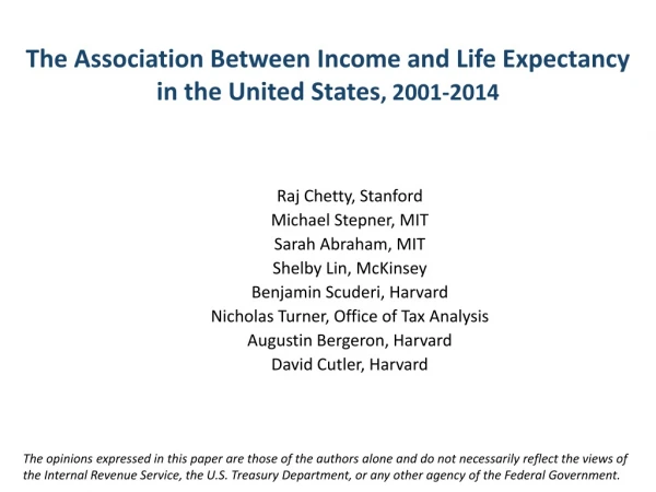
5. Improving Health Outcomes: Overview • This lecture illustrates how big data is helping us learn how to improve health, in three segments: • Descriptive analysis of health outcomes in U.S. population [method: survival analysis] Chetty, Stepner, Abraham, Lin, Scuderi, Bergeron, Cutler. “The Association Between Income and Life Expectancy in the United States” JAMA 2016.

6. Improving Health Outcomes: Overview • This lecture illustrates how big data is helping us learn how to improve health, in three segments: • Descriptive analysis of health outcomes in U.S. population [method: survival analysis] • Epidemiology application: using big data to forecast pandemics [method: predictive modeling] Ginsberg, Mohebbi, Patel, Brammer, Smolinski, Brilliant. “Detecting Influenza Epidemics Using Search Engine Query Data.” Nature 2009. Lazer, Kennedy, King, Vespignani. “The Parable of Google Flu: Traps in Big Data Analysis.” Science 2014.

7. Improving Health Outcomes: Overview • This lecture illustrates how big data is helping us learn how to improve health, in three segments: • Descriptive analysis of health outcomes in U.S. population [method: survival analysis] • Epidemiology application: using big data to forecast pandemics [method: predictive modeling] • Economics applications: impacts of health insurance coverage[method: regression discontinuities] Wherry, Miller, Kaestner, Meyer. “Childhood Medicaid Coverage and Later Life Health Care Utilization” REStat 2017.

8. Income and Life Expectancy • Most common measure of health: mortality rates • Crude but well measured in population data • Begin with basic descriptive facts about life expectancy in America • Chetty et al. (2016) examine relationship between life expectancy and income • Use data on entire U.S. population from 1999-2013 (1.4 billion observations)

9. Estimating Life Expectancy: Data • Mortality measured using Social Security death records • Income measured at household level using tax returns • Focus on percentile ranks in income distribution • Rank individuals in national income distribution within birth cohort, gender, and tax year

10. Methodology to Estimate Life Expectancy • Goal: estimate expected age of death conditional on an individual’s income at age 40, controlling for differences in race and ethnicity • Period life expectancy: life expectancy for a hypothetical individual who experiences mortality rates at each age observed in a given year • Three steps: • Calculate mortality rates by income rank and age for observed ages • Estimate a survival model to extrapolate to older ages • Adjust for racial differences in mortality rates

11. Survival Curve for Men at 5th Percentile 100 Age 76 80 60 Survival Rate (%) 40 20 0 40 60 80 100 120 Age in Years (a)

12. Survival Curves for Men at 5th and 95th Percentiles 100 Age 76 80 60 Survival Rate (%) 40 20 0 40 60 80 100 120 Age in Years (a)

13. Survival Curves for Men at 5th and 95th Percentiles 100 Age 76 80 p95 Survival Rate: 83% 60 Survival Rate (%) p5 Survival Rate: 52% 40 20 0 40 60 80 100 120 Age in Years (a)

14. Step 2: Predicting Mortality Rates at Older Ages • To calculate life expectancy, need estimates of mortality rates beyond age 76 • Gompertz (1825) documented a robust empirical pattern: mortality rates grow exponentially with age

15. Mortality Rates by Gender in the United States in 2001: CDC Data 0 -2 Log Mortality Rate -4 -6 40 50 60 70 80 90 100 Age in Years Age 76 Men Women

16. Log Mortality Rates for Men at 5th and 95th Percentiles -2 -4 Log Mortality Rate -6 -8 40 50 60 70 80 90 Age in Years Data: p5 Gompertz: p5 Data: p95 Gompertz: p95

17. Log Mortality Rates for Men at 5th and 95th Percentiles -2 -4 Log Mortality Rate -6 -8 40 50 60 70 80 90 Age in Years Age 65 Medicare Eligibility Threshold Data: p5 Gompertz: p5 Data: p95 Gompertz: p95

18. Survival Curves for Men at 5th and 95th Percentiles 100 Age 76 Age 90 80 60 Survival Rate (%) 40 20 Gompertz Extrapolation 0 40 60 80 100 120 Age in Years (a) Data: p5 Gompertz: p5 Data: p95 Gompertz: p95

19. Survival Curves for Men at 5th and 95th Percentiles 100 Age 76 Age 90 80 60 Survival Rate (%) 40 NCHS and SSA Estimates (constant across 20 income groups) Gompertz Extrapolation 0 40 60 80 100 120 Age in Years (a) Data: p5 Gompertz: p5 Data: p95 Gompertz: p95

20. Race and Ethnicity Adjustment • CDC data: for males, life expectancy of whites is 3.8 years higher than blacks and 2.7 years lower than Hispanics • Adjust for such racial and ethnic differences as follows: • Use National Longitudinal Mortality Study to estimate racial and ethnic differences in mortality rates by age, controlling for income • Use Census data to construct race- and ethnicity-adjusted estimates of life expectancy, to answer the question: “What would life expectancy be if each income group and area had the same black, Hispanic and Asian shares as the U.S. population as a whole at age 40?”

21. National Statistics on Income and Life Expectancy

22. Expected Age at Death vs. Household Income Percentile For Men at Age 40 90 85 Expected Age at Death for 40 Year Olds in Years 80 75 70 0 20 $25k 40 $47k 60 $74k 80 $115k 100 $2.0M Household Income Percentile

23. Expected Age at Death vs. Household Income Percentile For Men at Age 40 90 85 Expected Age at Death for 40 Year Olds in Years 80 75 70 0 20 $25k 40 $47k 60 $74k 80 $115k 100 $2.0M Household Income Percentile Top 1%: 87.3 Years Bottom 1%: 72.7 Years

24. U.S. Life Expectancies by Percentile in Comparison to Mean Life Expectancies Across Countries United States - P100 San Marino United States - P50 Canada United Kingdom United States - P25 China Libya Pakistan United States - P1 Sudan Iraq India Zambia Lesotho 60 65 70 75 80 85 90 Expected Age at Death for 40 Year Old Men

25. Expected Age at Death vs. Household Income Percentile By Gender at Age 40 90 Women 85 Men Expected Age at Death for 40 Year Olds in Years 80 75 Women, Bottom 1%: 78.8 Women, Top 1%: 88.9 Men, Bottom 1%: 72.7 Men, Top 1%: 87.3 70 0 20 40 60 80 100 Household Income Percentile

26. Expected Age at Death vs. Household Income Percentile By Gender at Age 40 90 85 Expected Age at Death for 40 Year Olds in Years 80 75 Women, Bottom 1%: 78.8 Women, Top 1%: 88.9 Men, Bottom 1%: 72.7 Men, Top 1%: 87.3 70 0 20 40 60 80 100 Household Income Percentile Top 1% Gender Gap 1.6 years Bottom 1% Gender Gap 6.1 years

27. Time Trends • How are gaps in life expectancy changing over time?

28. Trends in Expected Age at Death by Income Quartile in the US For Men Age 40, 2001-2014 90 Annual Change = 0.20 (0.17, 0.24) Annual Change = 0.18 (0.15, 0.20) 85 Expected Age at Death for 40 Year Olds in Years Annual Change = 0.12 (0.08, 0.16) 80 Annual Change = 0.08 (0.05, 0.11) 75 2000 2005 2010 2015 Year 1st Quartile 2nd Quartile 3rd Quartile 4th Quartile

29. Trends in Expected Age at Death by Income Quartile in the US For Women Age 40, 2001-2014 90 Annual Change = 0.23 (0.20, 0.25) Annual Change = 0.25 (0.22, 0.28) 88 Annual Change = 0.17 (0.13, 0.20) Expected Age at Death for 40 Year Olds in Years 86 84 Annual Change = 0.10 (0.06, 0.13) 82 2000 2005 2010 2015 Year 1st Quartile 2nd Quartile 3rd Quartile 4th Quartile

30. Local Area Variation in Life Expectancy by Income

31. Expected Age at Death vs. Household Income for Men in Selected Cities 90 85 New York City 80 San Francisco Dallas 75 Detroit 70 0 25 50 75 100 $30k $60k $101k $683k Household Income Percentile

32. Expected Age at Death vs. Household Income for Women in Selected Cities 90 85 New York City San Francisco Dallas 80 Detroit 75 70 0 50 75 100 $27k $54k $95k $653k Household Income Percentile

33. Expected Age at Death for 40 Year Old Men Bottom Quartile of U.S. Income Distribution Note: Lighter Colors Represent Areas with Higher Life Expectancy

34. Expected Age at Death for 40 Year Old Men Pooling All Income Groups Note: Lighter Colors Represent Areas with Higher Life Expectancy

35. Expected Age at Death for 40 Year Old Women Bottom Quartile of U.S. Income Distribution Note: Lighter Colors Represent Areas with Higher Life Expectancy

36. Expected Age at Death for 40 Year Olds in Bottom Quartile Top 10 and Bottom 10 CZs Among 100 Largest CZs Note: 95% confidence intervals shown in parentheses

37. Local Area Variation in Trends • Next, analyze how trends in life expectancy vary across areas

38. Change in Expected Age at Death in Bottom Quartile Birmingham, AL 90 Annual Change = 0.37 (0.20, 0.55) 85 Expected Age at Death in Years 80 75 Annual Change = 0.20 (0.07, 0.35) 70 2001 2014 Year Men Women

39. Change in Expected Age at Death in Bottom Quartile Birmingham, AL Tampa, FL 90 Annual Change = 0.37 (0.20, 0.55) Annual Change = -0.18 (-0.30, -0.06) 85 Women Expected Age at Death in Years 80 Men 75 Annual Change = 0.20 (0.07, 0.35) Annual Change = -0.16 (-0.25, -0.07) 70 2001 2014 2001 2014 Year Men Women

40. Change in Expected Age at Death in Bottom Quartile Top 10 and Bottom 10 CZs Among 100 Largest CZs Note: 95% confidence intervals shown in parentheses

41. Correlates of Spatial Variation in Life Expectancy

42. Why Does Life Expectancy Vary Across Areas? • Finally, we characterize the features of areas with high vs. low life expectancy conditional on income

43. Correlations of Expected Age at Death with Health and Social Factors For Individuals in Bottom Quartile of Income Distribution

44. Smoking Rates for Individuals in Bottom Income Quartile Note: Lighter Colors Represent Areas Lower Smoking Rates

45. Correlations of Expected Age at Death with Health and Social Factors For Individuals in Bottom Quartile of Income Distribution

46. Correlations of Expected Age at Death with Other Factors For Individuals in Bottom Quartile of Income Distribution

47. Correlations: Summary • General pattern: Low-income people in affluent, educated cities live longer (and have healthier behaviors) • Why is this the case? • Spillovers from rich to poor: regulation, public revenues/transfers • Exposure to people with healthier behaviors • Sorting: low-income people who live in expensive cities are a selected group with different characteristics

48. Income and Life Expectancy: Lessons • Disparities in life expectancy are large and growing, but not immutable: • Some areas in the U.S. have relatively small and shrinking gaps • Reducing health disparities likely to require local interventions • Ex: targeted efforts to improve health among low-income individuals in specific cities such as Las Vegas and Detroit • Changing health behaviors at local level likely to be important • Trends imply that indexing eligibility for Social Security and Medicare to average life expectancy will amplify inequality

49. How Can We Improve Population Health? • Two types of approaches, with different questions and methods: • Public health interventions to change behaviors such as smoking, exercise, water quality, and spread of diseases • Provision of health care and health insurance • Illustrate frontier of research using big data in each of these areas using recent examples

50. Forecasting Pandemics • Classic problem in population health: forecasting and preventing health pandemics • Contagious diseases like flu spread exponentially  large returns to taking action quickly when disease emerges • Most common method to monitor contagious diseases in developed countries: aggregated data from local clinics • Problem: slow reporting and small samples  data not very fine-grained