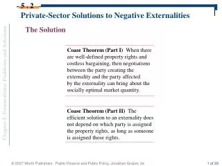
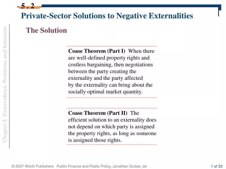
Private-Sector Solutions to Negative Externalities

1. Private-Sector Solutions to Negative Externalities 5 . 2 The Solution Coase Theorem (Part I) When there are well-defined property rights and costless bargaining, then negotiations between the party creating the externality and the party affected by the externality can bring about the socially optimal market quantity. Coase Theorem (Part II) The efficient solution to an externality does not depend on which party is assigned the property rights, as long as someone is assigned those rights.

2. 5 . 2 Example I Net Benefit to the factory associated with marginal production = $1.0 Net Cost to the Laundromat associated with the firm’s marginal production = $1.20 *Efficient outcome? Case (i): Factory has the property right. Case (ii): Laundromat has the property right

3. 5 . 2 Example II Net Benefit to the factory associated with marginal production = $1.20 Net Cost to the Laundromat associated with the firm’s marginal production = $1.0 *Efficient outcome? Case (i): Factory has the property right Case (ii): Laundromat has the property right

4. 5 . 2 The problem of the Common Example: 1000 identical persons who can do nothing but fish. Each can catch 4 fish on shore. * * *

5. Distinctions Between Price and Quantity Approaches to Addressing Externalities 5 . 4 Basic Model

6. Abatement: Algebraic Illustration Ē = firm’s pollution without abatement X = abatement E = Ē-X = pollution C(X) = abatement cost D(E) = D(Ē–X) = pollution damage C’(X) = marginal abatement cost D’(E) = marginal damage of pollution

7. 1. Optimal abatement: Choose X to Minimize C(X) + D(E) = C(X) + D(Ē-X) => C’(X) - D’(Ē-X)=0. Or, C’(X) = D’(E).

8. 2. Optimal solution for a firm in the presence of a tax: Minimize C(X) + t E = C(X) + t Ē – t X (x) => t= C’(x) To attain social optimum then, set t= D’(E).

9. Distinctions Between Price and Quantity Approaches to Addressing Externalities 5 . 4 Multiple Plants with Different Reduction Costs

10. Example with Multiple Firms Ē1, Ē2; X1, X2; E1 = Ē1 - X1; E2 = Ē2 - X2 Pollution damage = D(E1+E2) =D(Ē1 + Ē2 - X1 - X2)

11. * Optimal abatement: Minimize C1(X1) + C2(X2) + D(Ē1 + Ē2 - X1 - X2) C1’ (X1) = C2’(X2) = D’(E). * Firm’s solution: Minimizes Ci(Xi) + t (Ēi - Xi) => Ci’(Xi) = t. => Set: t = D’(E)

12. Example Assume: D(E) =10 E => D’(E) =10 C1(X1)=F + 1/10 (X1)2 => C1’(X1) =1/5 (X1) C2(X2)=F + 1/30 (X2)2 => C2’(X2) =1/15 (X2) Setting C1’(X1) = C2’(X2) = D’(E) => X1=50; X2=150

13. Equal pollution Reduction: Ask each firm to reduce pollution by 100. Same benefit of damage reduction as with the Pigouvian solution. Costs: C1 = F + 1/10 (100)2 C2 = F + 1/30 (100)2

14. Total cost of abatement= C1 + C2 = 2F + (100)2 [1/10 + 1/30] = 2F + 4000/3 Versus the total cost for the Pigouvian solution: C1 = F + 1/10 (50)2 C2 = F + 1/30 (150)2 => C1 +C2 = 2F + 1000.

15. Market for Permits Suppose Ē1 + Ē2 = 500. Want 200 reduction Issue 300 permits (150 each) Firm i’s pollution level is Ei = Ēi - Xi = 150 + ni ni denotes the number of extra permits purchased. If ni is negative, it will be the number of permits sold.

16. Price of a permit= p Cost of polluting Ei = Ci (Xi) + ni p Or Ci (Xi) + (Ē - Xi – 150) p Minimizing costs yields Ci’(Xi)=p. C1’(X1)= C2’(X2) If p=t, we will have the Pigouvian solution.