Download
1 / 49
500 likes | 583 Views
CS 4102 – Algorithms Dynamic programming Also, memoization Examples: Longest Common Subsequence Readings: 8.1, pp. 334-335, 8.4, p. 361 Also, handout on 0/1 knapsack Wikipedia articles. Dynamic programming. Old “bad” name (see Wikipedia or Notes, p. 361)

E N D
CS 4102 – Algorithms • Dynamic programming • Also, memoization • Examples: • Longest Common Subsequence • Readings: 8.1, pp. 334-335, 8.4, p. 361 • Also, handout on 0/1 knapsack • Wikipedia articles
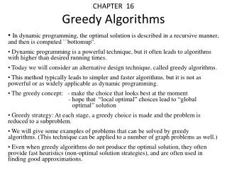
Dynamic programming • Old “bad” name (see Wikipedia or Notes, p. 361) • It is used, when the solution can be recursively described in terms of solutions to subproblems (optimal substructure) • Algorithm finds solutions to subproblems and stores them in memory for later use • More efficient than “brute-force methods”, which solve the same subproblems over and over again
Optimal Substructure Property • Definition on p. 334 • If S is an optimal solution to a problem, then the components of S are optimal solutions to subproblems • Examples: • True for knapsack • True for coin-changing (p. 334) • True for single-source shortest path • Not true for longest-simple-path (p. 335)
Dynamic Programming • Works “bottom-up” • Finds solutions to small sub-problems first • Stores them • Combines them somehow to find a solution to a slightly larger subproblem • Compare to greedy approach • Also requires optimal substructure • But greedy makes choice first, then solves
Problems Solved with Dyn. Prog. • Coin changing (Section 8.2, we won’t do) • Multiplying a sequence of matrices (8.3, we might do if we have time) • Can do in various orders: (AB)C vs. A(BC) • Pick order that does fewest number of scalar multiplications • Longest common subsequence (8.4, we’ll do) • All-pairs shortest paths (Floyd’s algorithm) • Remember from CS216? • Constructing optimal binary search trees • Knapsack problems (we’ll do 0/1)
Remember Fibonacci numbers? • Recursive code:long fib(int n) { assert(n >= 0); if ( n == 0 ) return 0; if ( n == 1 ) return 1; return fib(n-1) + fib(n-2); } • What’s the problem? • Repeatedly solves the same subproblems • “Obscenely” exponential (p. 326)
Memoization • Before talking about dynamic programming, another general technique: Memoization • AKA using a memory function • Simple idea: • Calculate and store solutions to subproblems • Before solving it (again), look to see if you’ve remembered it
Memoization • Use a Table abstract data type • Lookup key: whatever identifies a subproblem • Value stored: the solution • Could be an array/vector • E.g. for Fibonacci, store fib(n) usingindex n • Need to initialize the array • Could use a map / hash-table
Memoization and Fibonacci • Before recursive code below called, must initialize results[] so all values are -1long fib_mem(int n, long results[]) { if ( results[n] != -1 ) return results[n]; // return stored value long val; if ( n == 0 || n ==1 ) val = n; // odd but rightelse val = fib_mem(n-1, results) + fib_mem(n-2, results); results[n] = val; // store calculated value return val; }
Observations on fib_mem() • Same elegant top-down, recursive approach based on definition • Without repeated subproblems • Memory function: a function that remembers • Save time by using extra space • Can show this runs in (n)
Memoization and Functional Languages • Languages like Lisp and Scheme are functional languages • How could memoization help? • What could go wrong? Would this always work? • Side effects • Haskell does this (call-by-need)
General Strategy of Dyn. Prog. • Structure: What’s the structure of an optimal solution in terms of solutions to its subproblems? • Give a recursive definition of an optimal solution in terms of optimal solutions to smaller problems • Usually using min or max • Use a data structure (often a table) to store smaller solutions in a bottom-up fashion • Optimal value found in the table • (If needed) Reconstruct the optimal solution • I.e. what produced the optimal value
Dyn. Prog. vs. Divide and Conquer • Remember D & C? • Divide into subproblems. Solve each. Combine. • Good when subproblems do not overlap, when they’re independent • No need to repeat them • Divide and conquer: top-down • Dynamic programming: bottom-up
LCS: Section 8.4 • A “significant” example • Lots of detail • Look at example here and the one in the book
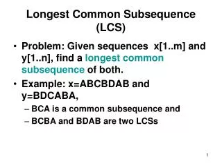
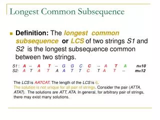
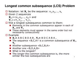
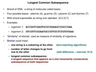
Longest Common Subsequence (LCS) Application: comparison of two DNA strings Ex: X= {A B C B D A B }, Y= {B D C A B A} Longest Common Subsequence: X = A BCB D A B Y = B D C A BA Brute force algorithm would compare each subsequence of X with the symbols in Y
LCS Algorithm • if |X| = m, |Y| = n, then there are 2m subsequences of X; we must compare each with Y (n comparisons) • So the running time of the brute-force algorithm is O(n 2m) • Notice that the LCS problem has optimal substructure: solutions of subproblems are parts of the final solution. • Subproblems: “find LCS of pairs of prefixes of X and Y”
LCS Algorithm • First we’ll find the length of LCS. Later we’ll modify the algorithm to find LCS itself. • Define Xi, Yj to be the prefixes of X and Y of length i and j respectively • Define c[i,j] to be the length of LCS of Xi and Yj • Then the length of LCS of X and Y will bec[m,n]
LCS recursive solution • We start with i = j = 0 (empty substrings of x and y) • Since X0 and Y0 are empty strings, their LCS is always empty (i.e. c[0,0] = 0) • LCS of empty string and any other string is empty, so for every i and j: c[0, j] = c[i,0] = 0
LCS recursive solution • When we calculate c[i,j], we consider two cases: • First case:x[i]=y[j]: one more symbol in strings X and Y matches, so the length of LCS Xi and Yjequals to the length of LCS of smaller strings Xi-1 and Yi-1 , plus 1
LCS recursive solution • Second case:x[i] != y[j] • As symbols don’t match, our solution is not improved, and the length of LCS(Xi , Yj) is the same as before (i.e. maximum of LCS(Xi, Yj-1) and LCS(Xi-1,Yj) Why not just take the length of LCS(Xi-1, Yj-1) ?
LCS Length Algorithm LCS-Length(X, Y) 1. m = length(X) // get the # of symbols in X 2. n = length(Y) // get the # of symbols in Y 3. for i = 1 to m c[i,0] = 0 // special case: Y0 4. for j = 1 to n c[0,j] = 0 // special case: X0 5. for i = 1 to m // for all Xi 6. for j = 1 to n // for all Yj 7. if ( Xi == Yj ) 8. c[i,j] = c[i-1,j-1] + 1 9. else c[i,j] = max( c[i-1,j], c[i,j-1] ) 10. return c[m,n] // return LCS length for X and Y
LCS Example We’ll see how LCS algorithm works on the following example: • X = ABCB • Y = BDCAB What is the Longest Common Subsequence of X and Y? LCS(X, Y) = BCB X = A BCB Y = B D C A B
ABCB BDCAB LCS Example (0) j 0 1 2 3 4 5 i Yj B D C A B Xi 0 A 1 B 2 3 C 4 B X = ABCB; m = |X| = 4 Y = BDCAB; n = |Y| = 5 Allocate array c[5,4]
ABCB BDCAB LCS Example (1) j 0 1 2 3 4 5 i Yj B D C A B Xi 0 0 0 0 0 0 0 A 1 0 B 2 0 3 C 0 4 B 0 for i = 1 to m c[i,0] = 0 for j = 1 to n c[0,j] = 0
ABCB BDCAB LCS Example (2) j 0 1 2 3 4 5 i Yj B D C A B Xi 0 0 0 0 0 0 0 A 1 0 0 B 2 0 3 C 0 4 B 0 if ( Xi == Yj ) c[i,j] = c[i-1,j-1] + 1 else c[i,j] = max( c[i-1,j], c[i,j-1] )
ABCB BDCAB LCS Example (3) j 0 1 2 3 4 5 i Yj B D C A B Xi 0 0 0 0 0 0 0 A 1 0 0 0 0 B 2 0 3 C 0 4 B 0 if ( Xi == Yj ) c[i,j] = c[i-1,j-1] + 1 else c[i,j] = max( c[i-1,j], c[i,j-1] )
ABCB BDCAB LCS Example (4) j 0 1 2 3 4 5 i Yj B D C A B Xi 0 0 0 0 0 0 0 A 1 0 0 0 0 1 B 2 0 3 C 0 4 B 0 if ( Xi == Yj ) c[i,j] = c[i-1,j-1] + 1 else c[i,j] = max( c[i-1,j], c[i,j-1] )
ABCB BDCAB LCS Example (5) j 0 1 2 3 4 5 i Yj B D C A B Xi 0 0 0 0 0 0 0 A 1 0 0 0 0 1 1 B 2 0 3 C 0 4 B 0 if ( Xi == Yj ) c[i,j] = c[i-1,j-1] + 1 else c[i,j] = max( c[i-1,j], c[i,j-1] )
ABCB BDCAB LCS Example (6) j 0 1 2 3 4 5 i Yj B D C A B Xi 0 0 0 0 0 0 0 A 1 0 0 0 0 1 1 B 2 0 1 3 C 0 4 B 0 if ( Xi == Yj ) c[i,j] = c[i-1,j-1] + 1 else c[i,j] = max( c[i-1,j], c[i,j-1] )
ABCB BDCAB LCS Example (7) j 0 1 2 3 4 5 i Yj B D C A B Xi 0 0 0 0 0 0 0 A 1 0 0 0 0 1 1 B 2 0 1 1 1 1 3 C 0 4 B 0 if ( Xi == Yj ) c[i,j] = c[i-1,j-1] + 1 else c[i,j] = max( c[i-1,j], c[i,j-1] )
ABCB BDCAB LCS Example (8) j 0 1 2 3 4 5 i Yj B D C A B Xi 0 0 0 0 0 0 0 A 1 0 0 0 0 1 1 B 2 0 1 1 1 1 2 3 C 0 4 B 0 if ( Xi == Yj ) c[i,j] = c[i-1,j-1] + 1 else c[i,j] = max( c[i-1,j], c[i,j-1] )
ABCB BDCAB LCS Example (10) j 0 1 2 3 4 5 i Yj B D C A B Xi 0 0 0 0 0 0 0 A 1 0 0 0 0 1 1 B 2 0 1 1 1 1 2 3 C 0 1 1 4 B 0 if ( Xi == Yj ) c[i,j] = c[i-1,j-1] + 1 else c[i,j] = max( c[i-1,j], c[i,j-1] )
ABCB BDCAB LCS Example (11) j 0 1 2 3 4 5 i Yj B D C A B Xi 0 0 0 0 0 0 0 A 1 0 0 0 0 1 1 B 2 0 1 1 1 1 2 3 C 0 1 1 2 4 B 0 if ( Xi == Yj ) c[i,j] = c[i-1,j-1] + 1 else c[i,j] = max( c[i-1,j], c[i,j-1] )
ABCB BDCAB LCS Example (12) j 0 1 2 3 4 5 i Yj B D C A B Xi 0 0 0 0 0 0 0 A 1 0 0 0 0 1 1 B 2 0 1 1 1 1 2 3 C 0 1 1 2 2 2 4 B 0 if ( Xi == Yj ) c[i,j] = c[i-1,j-1] + 1 else c[i,j] = max( c[i-1,j], c[i,j-1] )
ABCB BDCAB LCS Example (13) j 0 1 2 3 4 5 i Yj B D C A B Xi 0 0 0 0 0 0 0 A 1 0 0 0 0 1 1 B 2 0 1 1 1 1 2 3 C 0 1 1 2 2 2 4 B 0 1 if ( Xi == Yj ) c[i,j] = c[i-1,j-1] + 1 else c[i,j] = max( c[i-1,j], c[i,j-1] )
ABCB BDCAB LCS Example (14) j 0 1 2 34 5 i Yj B D C A B Xi 0 0 0 0 0 0 0 A 1 0 0 0 0 1 1 B 2 0 1 1 1 1 2 3 C 0 1 1 2 2 2 4 B 0 1 1 2 2 if ( Xi == Yj ) c[i,j] = c[i-1,j-1] + 1 else c[i,j] = max( c[i-1,j], c[i,j-1] )
ABCB BDCAB LCS Example (15) j 0 1 2 3 4 5 i Yj B D C A B Xi 0 0 0 0 0 0 0 A 1 0 0 0 0 1 1 B 2 0 1 1 1 1 2 3 C 0 1 1 2 2 2 3 4 B 0 1 1 2 2 if ( Xi == Yj ) c[i,j] = c[i-1,j-1] + 1 else c[i,j] = max( c[i-1,j], c[i,j-1] )
LCS Algorithm Running Time • LCS algorithm calculates the values of each entry of the array c[m,n] • So what is the running time? O(m*n) since each c[i,j] is calculated in constant time, and there are m*n elements in the array
How to find actual LCS • So far, we have just found the length of LCS, but not LCS itself. • We want to modify this algorithm to make it output Longest Common Subsequence of X and Y Each c[i,j] depends on c[i-1,j] and c[i,j-1] or c[i-1, j-1] For each c[i,j] we can say how it was acquired: For example, here c[i,j] = c[i-1,j-1] +1 = 2+1=3 2 2 2 3
How to find actual LCS - continued • Remember that • So we can start from c[m,n] and go backwards • Look first to see if 2nd case above was true • If not, then c[i,j] = c[i-1, j-1]+1, so remember x[i] (because x[i] is a part of LCS) • When i=0 or j=0 (i.e. we reached the beginning), output remembered letters in reverse order
Algorithm to find actual LCS • Here’s a recursive algorithm to do this:LCS_print(x, m, n, c) { if (c[m][n] == c[m-1][n]) // go up? LCS_print(x, m-1, n, c); else if (c[m][n] == c[m][n-1] // go left? LCS_print(x, m, n-1, c); else { // it was a match! LCS_print(x, m-1, n-1, c); print(x[m]); // print after recursive call }}
Finding LCS j 0 1 2 3 4 5 i Yj B D C A B Xi 0 0 0 0 0 0 0 A 1 0 0 0 0 1 1 B 2 0 1 1 1 1 2 3 C 0 1 1 2 2 2 3 4 B 0 1 1 2 2
Finding LCS (2) j 0 1 2 3 4 5 i Yj B D C A B Xi 0 0 0 0 0 0 0 A 1 0 0 0 0 1 1 B 2 0 1 1 1 1 2 3 C 0 1 1 2 2 2 3 4 B 0 1 1 2 2 B C B LCS (reversed order): B C B (this string turned out to be a palindrome) LCS (straight order):
Review: Dynamic programming • DP is a method for solving certain kind of problems • DP can be applied when the solution of a problem includes solutions to subproblems • We need to find a recursive formula for the solution • We can recursively solve subproblems, starting from the trivial case, and save their solutions in memory • In the end we’ll get the solution of the whole problem
Properties of a problem that can be solved with dynamic programming • Simple Subproblems • We should be able to break the original problem to smaller subproblems that have the same structure • Optimal Substructure of the problems • The solution to the problem must be a composition of subproblem solutions • Subproblem Overlap • Optimal subproblems to unrelated problems can contain subproblems in common
Review: Longest Common Subsequence (LCS) • Problem: how to find the longest pattern of characters that is common to two text strings X and Y • Dynamic programming algorithm: solve subproblems until we get the final solution • Subproblem: first find the LCS of prefixes of X and Y. • this problem has optimal substructure: LCS of two prefixes is always a part of LCS of bigger strings
Conclusion • Dynamic programming is a useful technique of solving certain kind of problems • When the solution can be recursively described in terms of partial solutions, we can store these partial solutions and re-use them as necessary • Running time (Dynamic Programming algorithm vs. naïve algorithm): • LCS: O(m*n) vs. O(n * 2m) • 0-1 Knapsack problem: O(W*n) vs. O(2n)