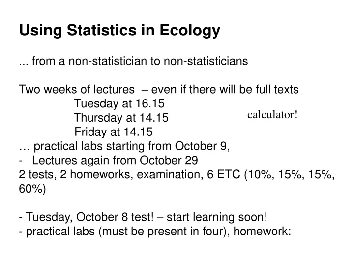
Using Statistics in Ecology ... from a non- statistician to non- statisticians

1. UsingStatistics in Ecology ... from a non-statisticianto non-statisticians Twoweeks of lectures – eveniftherewillbefulltexts Tuesday at 16.15 Thursday at 14.15 Friday at 14.15 … practicallabsstartingfromOctober 9, • LecturesagainfromOctober 29 2 tests, 2 homeworks, examination, 6 ETC (10%, 15%, 15%, 60%) - Tuesday, October 8 test! – start learning soon! • practicallabs (must be present in four), homework: calculator!

2. Solving tasks in Excel and R. Labmaster Jaanis Lodjak: jaanis.lodjak@gmail.com http://www.ut.ee/~tammarut/stat.htm toomas.tammaru@ut.ee

3. http://www.ut.ee/~tammarut/stateng.htm

4. Why do we need statistics (especially) in biology? …. a jar of sulfuric acid is a jar of sulfuric acid,

5. Why do we need statistics (especially) in biology? … a jar of sulfuric acid is a jar of sulfuric acid, ..... a mouse is this mouse.

6. Why do we need statistics (especially) in biology? …. a jar of sulfuric acid is a jar of sulfuric acid, ..... a mouse is this mouse. objects are not equal, individuality • individuals, parts of those, populations. ... but we usually want to conclude something about a class of objects in general. Statistics is needed to manage the clouds of individual variation and to see the general pattern through those What should we do then? We cannot study them all (population), we study a sample. The larger the better – statistics expresses it in numbers!

7. Describing sample and population A continuous vs discrete variable, objects and observations, observations form a distribution. Easy: a binary distribution Continuous distribution: histogram, density function is an abstraction. Normal distribution, • many factors affect; • strictly speaking, does not exist in reality, many variables have close-to natural distributions;

8. Describing samples and populations, Various parameters describing the average of the distribution: (Sample) mean (‘true mean’ of a population) – arithmetic mean; Median: equal number of observations smaller and larger; Mode: most common value. Coincide in the case of symmetric distribution, Example: distribution of income.

9. Measures of variability – different kinds, „more variable“ can be expressed in different ways. Variance an estimate of the variance of the population: representative! No difference when the sample is large; why bad: units are not the same; Why good: - additivity, can be decomposed into components.

10. body tail fish head total var Length of a fish is the sum of head, body and tail - components of variance sum up in the same way - so much of variance attributable to one, so much to another...

11. Standard deviation (SD) is square root of variance, • how many times is variation larger? - ± SD: 68% of observations, can be outside; Coefficient of variation, CV Quantilesorfractiles divide distribution to parts of certain size, 25% and 75% quantiles - quartiles. In case of normal distribution SD is interpretable as quantiles (16% ja 84%), not in general case. Values do not depend of sample size.

12. Similar but substantially different parameters characterize the accuracy of our knowledge about population mean. Standard error, SE, is calculated as SD/squareroot-N. Depens on variance and sample size. Confidence interval of the mean Is a parameter analogous to CV – it would be strange to have this interval outside of this interval, 95% usually, ± SE is a 68% confidence interval.

13. Please note: SE and confidence intervals characterise our knowledge about population mean, they are not meant to describe variability in the population, SE tends to zero with N increasing.

14. Variance in a sample: Estimate of variance in the population: kala pikkus, m fish length Estimate of SD in the population: square root of variance. Coefficient of variation: SD divided by the mean. Standard error SE: SD/squareroot-N.

15. mean 2, deviations: -1, 1, 0, 0 squares: 1, 1, 0, 0 Sum of squares: 2 variance = sum of squares/ N = 0.5 Estimate of variance of the population = 2/(4-1) = 0.66 Standard deviation = 0.816 CV: 40,8%, SE=0.408

16. Presenting measures of variability - with the ± sign mostly, - in figures, as error bar’s, you must tell what do you mean! SE error bars help us to evaluate statistical signifinance For asymmetrical distributions, use quantiles Especially when: 0,2 0,1 0,1 0,1 0,9 0,8 we will get 0.36±0.37, Median should be used with quantiles.

17. Box plotwhen several parameters at a time. Write down what is what! Ordinary bar plots when relative differences are of interest. More complex parameters - skewnesscharacterises asymmetry. Long tail to the right – skewness is positive. - kurtosis – positive when pointed.

18. Statistical test - we see a difference or a relationship in our sample; - can we claim that it exists in the population as well? - about the population based on a sample; Statistical significance pmeasures the probability to get the situation by chance, ... in the case when there isn’t … in the population.

19. Statistical significance expresses the probability to obtain (when taking samples from the population) a sample with a relationship with such a strength* in the case when actually there is no relationship in the population. * - „such a strength“ means the stength which was observed in our actual sample. Let’s build a (computer) game and examine this question! Let’s simulate the situation in which there is no relationship in the population.

20. We have a sample N = 7 and no more information there was a correlation between eye size and IQ IQ r = 0,5 eye

22. We have a sample N = 7 and no more information there was a correlation between eye size and IQ IQ r = 0,5 eye

23. How can we know whether we can believe that there is a correlation also in the population? We will study if we can get a sample with such a relationship by chance. If the probability of obtaining such a sample by chance is high, there is no reason to believe that there is a relationship in the population; if the probability is low, we have a reason to believe.

24. How do we know how probable is to get it by chance, i.e. in the situation when there is no relationship in the population? We will simulate the situation when there is no relationship in the population, and will simulate taking samples from such population, the samples will be taken as large as our actual sample is.

25. Let’s create, on a computer, a sample with no correlation: IQ let’s take samples from it at random, N=7 eye r=0,2 IQ eye

26. r=0,2 r=-0,3 IQ IQ IQ r=0,7 eye eye eye 2 1000 times 1 0,2 0,7 0 -0,3 r values

27. p = 0.15 frequency in 150 cases out of 1000, the r-value is larger than our actual one, it is quite likely to get our sample by chance, it would be too brave to conclude that there is a relationship in the population. -1 0 +1 r-values +0,5

28. A quite arbitrary limit p < 0,05 … in which case we say that the difference is statistically significant

29. p-value tells us how probable is to obtain the observed situation (difference or relationship) by chance, p-value does not tell us how probable it is that the relationship was obtained by chance, which means that p=0.02 cannot be interpreted so that „with a 2% probability the relationship was obtained by chance“ or that „with a 98% probability there actually is a relationship.“

30. Please note that the p value does not characterise the strength of the relationship! Statistical significance depends on: - strength of the relationship; - sample size; - on the amount of variability. Please also note that we cannot prove that there is no relationship in the the population, we rather just do not know which way it is; As well as p is never zero – we never have absolute certainty 0 < p ≤ 1

31. Also, there are no significant and non-significant relationships in nature, p does not characterise a relationship, it characterises our knowledge about the relationship!

32. Degreeof freedom (df) is an unintelligible term typically coming up in connection to statistical tests, the number of degrees of freedom of a systemtellsus howmanyindependentnumbersdowe need tofully describethesystem. A trialnglehasthreedegrees of freedom. A datasetisfullydescribedwhenweknowthemodel (a regressionline,forexample), and thedeviation of eachobservationfromthemodel. • bothhaveitsowndegrees of freedom: modeldf – complexity of themodel; errordf– amount of thedata. -itdepends on thesethingsifthefit of themodelcanbeascribedtochanceornot.

33. There are many types of statistical tests, specific to particular situations, mastering statistics at the applied level implies the ability to choose correct test and to interpret the results; Choosing the test – first thing: are the variables continuous or discrete? First dependent variable continuous; independent variable discrete. t-test two groups – pre-existing or man-made

34. First, calculatet-statistic,which the larger - the larger is the difference between the means; - the larger is the sample; - the smaller is the variability in the samples. On the basis of t, find p from a table, because we cannot calculate it directly, degrees of freedom are those of the model: df=n1+n2-2, model df are always 1 and no need to report those.

36. Report results as here: “There was a difference in the length of perches between lakes A and B (t=2.7; df=34; p=0.025)” or also “Food plant had no effect on growth rate of the larvae (t=0.17; df=52; p=0.37)”

37. Arvutame ühe näite: where ... but in this case s2=0.667 df=n1+n2-2 t = 1/ (0.816p(1/4+1/4)) = = 1/(0.816*0,707) = 1.73 df= 6 p>0.1 fish length

38. t = 1.73 p = 0.13

39. was before t = 1.73 p = 0.13 t = 3.46 p = 0.013

40. t = 3.46 p = 0.013

41. was before t = 3.46 p = 0.013 t = 1.73 p = 0.13

42. t = 1.73 p = 0.13

43. was before t = 1.73 p = 0.13 t = 2.65 p = 0.019

44. One-way analysis of variance ANOVA like a t-test but comparing more than two groups The groups can also be called levels, „the independent variable has three levels“ (e.g. Black lake, White lake, Cat lake)

45. +2 +2 +2 +1 +1 +1 0 0 0 - 2 - 2 - 2 Relies on decompositing variance into its components - 1) the variance of group means: 2) the variance of individual observations around group means (residual variance, error variance), or variance among levels and within levels. Can we explain the differences among groups by variability within groups?

46. situation 1 length situation 2 length

47. Will be formalised by calculating the F-statistic: F=MSmodel/MSerror MS=SS/df, mean square; SS is sum of squares. Squares of what? Of deviations. will find p on the basis of F, df are important; there are two df-s: df model and df-error, model df: k-1; error df: n-k

48. +2 +2 +2 +2 +1 +1 +1 +1 0 0 0 0 - 2 - 2 - 2 - 2 4 3 -1 2 -1 1 -1 -1 SS model = SS(1, 2, 3, 4)*5 = 25 SS error = SS( +1,+2,-1,-2, 0, +1,+2,-1,-2, 0,+1,+2,-1,-2, 0, +1,+2,-1,-2, 0) = 40 MS model= SS model /3 = 8.33 MS error = SS error /16 = 2.5 F = 8.33/2.5 = 3.33; p = 0.046

49. Coefficient of determination: R2 =SSmodel/SStotal, „the model explains (accounts for) …. % of variance“, characterises the effect of manipulation; We will write: “host plant had an effect on pupal weight (F3,16 = 3,33, p=0,046)”, but we do not know which one! also R2

50. R2 = 0 p = 1