Download
1 / 36
360 likes | 551 Views
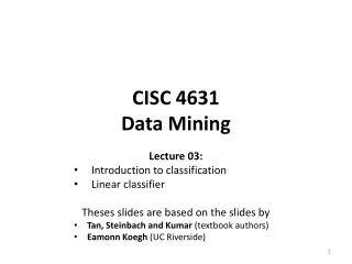
CISC 4631 Data Mining. Lecture 06: Bayes Theorem Theses slides are based on the slides by Tan, Steinbach and Kumar (textbook authors) Eamonn Koegh (UC Riverside) Andrew Moore (CMU/Google). Naïve Bayes Classifier. Thomas Bayes 1702 - 1761.

E N D
CISC 4631Data Mining Lecture 06: Bayes Theorem Theses slides are based on the slides by Tan, Steinbach and Kumar (textbook authors) EamonnKoegh(UC Riverside) Andrew Moore (CMU/Google)
Naïve Bayes Classifier Thomas Bayes 1702 - 1761 We will start off with a visual intuition, before looking at the math…
10 9 8 7 6 5 4 3 2 1 1 2 3 4 5 6 7 8 9 10 Grasshoppers Katydids Antenna Length Abdomen Length Remember this example? Let’s get lots more data…
10 9 8 7 6 5 4 3 2 1 1 2 3 4 5 6 7 8 9 10 Katydids Grasshoppers With a lot of data, we can build a histogram. Let us just build one for “Antenna Length” for now… Antenna Length
We can leave the histograms as they are, or we can summarize them with two normal distributions. Let us us two normal distributions for ease of visualization in the following slides…
We want to classify an insect we have found. Its antennae are 3 units long. How can we classify it? • We can just ask ourselves, give the distributions of antennae lengths we have seen, is it more probable that our insect is a Grasshopperor a Katydid. • There is a formal way to discuss the most probable classification… p(cj | d) = probability of class cj, given that we have observed d 3 Antennae length is 3
Bayes Classifier • A probabilistic framework for classification problems • Often appropriate because the world is noisy and also some relationships are probabilistic in nature • Is predicting who will win a baseball game probabilistic in nature? • Before getting the heart of the matter, we will go over some basic probability. • We will review the concept of reasoning with uncertainty also known as probability • This is a fundamental building block for understanding how Bayesian classifiers work • It’s really going to be worth it • You may find a few of these basic probability questions on your exam • Stop me if you have questions!!!!
Discrete Random Variables • A is a Boolean-valued random variable if Adenotes an event, and there is some degree of uncertainty as to whether Aoccurs. • Examples • A= The next patient you examine is suffering from inhalational anthrax • A= The next patient you examine has a cough • A= There is an active terrorist cell in your city
Probabilities • We write P(A) as “the fraction of possible worlds in which Ais true” • We could at this point spend 2 hours on the philosophy of this. • But we won’t.
Visualizing A Event space of all possible worlds P(A) = Area of reddish oval Worlds in which A is true Its area is 1 Worlds in which A is False
The Axioms Of Probability • 0 <= P(A) <= 1 • P(True) = 1 • P(False) = 0 • P(A or B) = P(A) + P(B) - P(A and B) The area of A can’t get any smaller than 0 And a zero area would mean no world could ever have A true
Interpreting the axioms • 0 <= P(A) <= 1 • P(True) = 1 • P(False) = 0 • P(A or B) = P(A) + P(B) - P(A and B) The area of A can’t get any bigger than 1 And an area of 1 would mean all worlds will have A true
A B Interpreting the axioms • 0 <= P(A) <= 1 • P(True) = 1 • P(False) = 0 • P(A or B) = P(A) + P(B) - P(A and B)
Interpreting the axioms • 0 <= P(A) <= 1 • P(True) = 1 • P(False) = 0 • P(A or B) = P(A) + P(B) - P(A and B) A P(A or B) B B P(A and B) Simple addition and subtraction
Another important theorem • 0 <= P(A) <= 1, P(True) = 1, P(False) = 0 • P(A or B) = P(A) + P(B) - P(A and B) From these we can prove: P(A) = P(A and B) + P(A and not B) A B
Conditional Probability • P(A|B) = Fraction of worlds in which Bis true that also have A true H = “Have a headache” F = “Coming down with Flu” P(H) = 1/10 P(F) = 1/40 P(H|F) = 1/2 “Headaches are rare and flu is rarer, but if you’re coming down with ‘flu there’s a 50-50 chance you’ll have a headache.” F H
F H Conditional Probability P(H|F) = Fraction of flu-inflicted worlds in which you have a headache = #worlds with flu and headache ------------------------------------ #worlds with flu = Area of “H and F” region ------------------------------ Area of “F” region = P(H and F) --------------- P(F) H = “Have a headache” F = “Coming down with Flu” P(H) = 1/10 P(F) = 1/40 P(H|F) = 1/2
Definition of Conditional Probability P(A and B) P(A|B) = ----------- P(B) Corollary: The Chain Rule P(A and B) = P(A|B) P(B)
F H Probabilistic Inference H = “Have a headache” F = “Coming down with Flu” P(H) = 1/10 P(F) = 1/40 P(H|F) = 1/2 One day you wake up with a headache. You think: “Drat! 50% of flus are associated with headaches so I must have a 50-50 chance of coming down with flu” Is this reasoning good?
F H Probabilistic Inference H = “Have a headache” F = “Coming down with Flu” P(H) = 1/10 P(F) = 1/40 P(H|F) = 1/2 P(F and H) = … P(F|H) = …
F H Probabilistic Inference H = “Have a headache” F = “Coming down with Flu” P(H) = 1/10 P(F) = 1/40 P(H|F) = 1/2
What we just did… P(A & B) P(A|B) P(B) P(B|A) = ----------- = --------------- P(A) P(A) This is Bayes Rule Bayes, Thomas (1763) An essay towards solving a problem in the doctrine of chances. Philosophical Transactions of the Royal Society of London, 53:370-418
Some more terminology • The Prior Probability is the probability assuming no specific information. • Thus we would refer to P(A) as the prior probability of even A occurring • We would not say that P(A|C) is the prior probability of A occurring • The Posterior probability is the probability given that we know something • We would say that P(A|C) is the posterior probability of A (given that C occurs)
Example of Bayes Theorem • Given: • A doctor knows that meningitis causes stiff neck 50% of the time • Prior probability of any patient having meningitis is 1/50,000 • Prior probability of any patient having stiff neck is 1/20 • If a patient has stiff neck, what’s the probability he/she has meningitis?
Menu Menu Menu Menu Menu Menu Menu Another Example of BT Bad Hygiene Good Hygiene • You are a health official, deciding whether to investigate a restaurant • You lose a dollar if you get it wrong. • You win a dollar if you get it right • Half of all restaurants have bad hygiene • In a bad restaurant, ¾ of the menus are smudged • In a good restaurant, 1/3 of the menus are smudged • You are allowed to see a randomly chosen menu
Menu Menu Menu Menu Menu Menu Menu Menu Menu Menu Menu Menu Menu Menu Menu Menu
Why Bayes Theorem at all? • Why modeling P(C|A) via P(A|C) • Why not model P(C|A) directly? • P(A|C)P(C) decomposition allows us to be “sloppy” • P(C) and P(A|C) can be trained independently
Crime Scene Analogy • Ais a crime scene. Cis a person who may have committed the crime • P(C|A)- look at the scene - who did it? • P(C)- who had a motive? (Profiler) • P(A|C)- could they have done it? (CSI - transportation, access to weapons, alibi)