Download
1 / 15
150 likes | 277 Views
Results from the GRAPE Model Atsushi KUROSAWA Research and Development Division, The Institute of Applied Energy (IAE) Shinbashi SY bldg., 1-14-2 Nishishinbashi, Minato, Tokyo 105-0003 JAPAN Phone (+81) 3-3508-8894 / Fax (+81) 3-3501-1735 E-mail : kurosawa@iae.or.jp

E N D
Results from the GRAPE Model Atsushi KUROSAWA Research and Development Division, The Institute of Applied Energy (IAE)Shinbashi SY bldg., 1-14-2 Nishishinbashi, Minato, Tokyo 105-0003 JAPANPhone (+81) 3-3508-8894 / Fax (+81) 3-3501-1735 E-mail : kurosawa@iae.or.jp Expert Meeting on Assessment of Contributions to Climate ChangeUK Met Office, Bracknell UKSeptember 25-27, 2002 The views are solely those of the individual author and do not represent organizational view of the Institute of Applied Energy
Outline [1] GRAPE MODEL AND CLIMATE MODULE [2] PHASE 2 RESULTS GLOBAL SCALE ASSESSMENT AND SENSITIVITY RUNS [3] SUMMARY
[1] GRAPE MODEL AND CLIMATE MODULE ENERGY Energy CostEnergy Trade Carbon Trade CO2,CH4,N2O (Fossil Fuel) ECONOMY CLIMATE Biomass Energy Landuse Related Cost Food Trade Carbon(Deforestation) CH4(Livestock,Rice)N2O(Fertilizer),etc Atmospheric Temperature IMPACT LAND USE
Sources Emissions Concentration → Rad. Forc. Temperature Fos.Fuel Consumption CO2 Em. CO2 Conc. Atmosphere Forest Livestock CH4 Em. CH4 Conc. Rad. Forcing Rice Field N2O Em. N2O Conc. Fos. Fuel Production Ocean Fertilized Soil Other GHGs Em. Chemical Industry CLIMATE CHANGE
[2] PHASE 2 RESULTS GLOBAL SCALE ASSESSMENT AND SENSITIVITY RUNS # Formulation Emissions to Concentrations CO2 - Four Box model CH4,N2O – One Box model Concentrations to Rad. Forcings IPCC WGI TAR Rad. Forcings to Temp. Change & SLR Two Box model # Evaluation Period 10 year step
# Sensitivity Run Past Emissions : EDGAR Future Emissions : IPCC SRES A2 Marker Start End Case 1 1890 2000 - default Case 2 1990 2100 Case 3 1890 2100
# Regional Contibution Assessment Example : Region A Contribution >>> Nature + Region A Emission Definition of Contribution = (change of param. in regional calculation) / (change of param. in global calculation) Start End
# Strength of Non-Linearity -- Regional sum is not equal to 100%. Parameter Period (Reg.Sum) – (Global) CO2 Conc. Past (case 1) -15% Future (case 2) -31% Past+Future (case 3) -3%Rad Forcing Past -14% Future -37% Past+Future 25% Temp Past 5% Future -31% Past+Future 25% SLR Past 39% Future 31% Past+Future 30%
[3] SUMMARY # Strong non-linearity is observed. # Treatment of natural emission? # Historical evaluation start date should be 1760 as default value since this period is considered as the beginning of human interventions.