Download
1 / 30
300 likes | 433 Views
Class 9: Phylogenetic Trees. The Tree of Life. D’après Ernst Haeckel, 1891. Evolution. Many theories of evolution Basic idea: speciation events lead to creation of different species Speciation caused by physical separation into groups where different genetic variants become dominant

E N D
The Tree of Life D’après Ernst Haeckel, 1891
Evolution • Many theories of evolution • Basic idea: • speciation events lead to creation of different species • Speciation caused by physical separation into groups where different genetic variants become dominant • Any two species share a (possibly distant) common ancestor
Phylogenies • A phylogeny is a tree that describes the sequence of speciation events that lead to the forming of a set of current day species • Leafs - current day species • Nodes - hypothetical most recent common ancestors • Edges length - “time” from one speciation to the next Aardvark Bison Chimp Dog Elephant
Until mid 1950’s phylogenies were constructed by experts based on their opinion (subjective criteria) • The Linnaeus classification scheme implicitly assumes tree structure • Since then, focus on objective criteria for constructing phylogenetic trees • Thousands of articles in the last decades • Important for many aspects of biology • Classification (systematics) • Understanding biological mechanisms
Morphological vs. Molecular • Classical phylogenetic analysis: morphological features • number of legs, lengths of legs, etc. • Modern biological methods allow to use molecular features • Gene sequences • Protein sequences • Analysis based on homologous sequences (e.g., globins) in different species
Dangers in Molecular Phylogenies • We have to remember that gene/protein sequence can be homologous for different reasons: • Orthologs -- sequences diverged after a speciation event • Paralogs -- sequences diverged after a duplication event • Xenologs -- sequences diverged after a horizontal transfer (e.g., by virus)
Dangers of Paralogues Gene Duplication Speciation events 2B 1B 3A 3B 2A 1A
Dangers of Paralogs • If we only consider 1A, 2B, and 3A... Gene Duplication Speciation events 2B 1B 3A 3B 2A 1A
Types of Trees • A natural model to consider is that of rooted trees Common Ancestor
Types of Trees • Depending on the model, data from current day species does not distinguish between different placements of the root vs
Types of trees • Unrooted tree represents the same phylogeny with out the root node
Positioning Roots in Unrooted Trees • We can estimate the position of the root by introducing an outgroup: • a set of species that are definitely distant from all the species of interest Proposed root Falcon Aardvark Bison Chimp Dog Elephant
Type of Data • Distance-based • Input is a matrix of distances between species • Can be fraction of residue they disagree on, or alignment score between them, or … • Character-based • Examine each character (e.g., residue) separately
Simple Distance-Based Method Input: distance matrix between species Outline: • Cluster species together • Initially clusters are singletons • At each iteration combine two “closest” clusters to get a new one
UPGMA Clustering • Let Ci and Cj be clusters, define distance between them to be • When we combine two cluster, Ci and Cj, to form a new cluster Ck, then
Molecular Clock • UPGMA implicitly assumes that all distances measure time in the same way 2 3 2 3 4 1 4 1
Additivity • A weaker requirement is additivity • In “real” tree, distances between species are the sum of distances between intermediate nodes k c b j a i
Consequences of Additivity • Suppose input distances are additive • For any three leaves • Thus k c b j a m i
Neighbor Joining • Can we use this fact to construct trees? • Let where Theorem: if D(i,j) is minimal (among all pairs of leaves), then i and j are neighbors in the tree
Neighbor Joining • Set L to contain all leaves Iteration: • Choose i,j such that D(i,j) is minimal • Create new node k, and set • remove i,j from L, and add k Terminate:when |L| =2, connect two remaining nodes
Distance Based Methods • If we make strong assumptions on distances, we can reconstruct trees • In real-life distances are not additive • Sometimes they are close to additive
Parsimony • Character-based method Assumptions: • Independence of characters (no interactions) • Best tree is one where minimal changes take place
Simple Example • Suppose we have five species, such that three have ‘C’ and two ‘T’ at a specified position • Minimal tree has one evolutionary change: C T C T C C C T T C
Aardvark Bison Chimp Dog Elephant Another Example • What is the parsimony score of A: CAGGTA B: CAGACA C: CGGGTA D: TGCACT E: TGCGTA
Evaluating Parsimony Scores • How do we compute the Parsimony score for a given tree? • Weighted Parsimony • Each change is weighted by the score c(a,b)
Evaluating Parsimony Scores Dynamic programming on the tree Initialization: • For each leaf i set S(i,a) = 0 if i is labeled by a, otherwise S(i,a) = Iteration: • if k is node with children i and j, then S(k,a) = minb(S(i,b)+c(a,b)) + minb(S(j,b)+c(a,b)) Termination: • cost of tree is minaS(r,a) where r is the root
Aardvark Bison Chimp Dog Elephant Example A: CAGGTA B: CAGACA C: CGGGTA D: TGCACT E: TGCGTA
Cost of Evaluating Parsimony • If there are n nodes, m characters, and k possible values for each character, then complexity is O(nmk) • Using this procedure, we can reconstruct most parsimonious values at each ancestor node