Download
1 / 66
660 likes | 666 Views
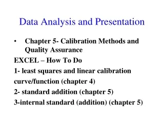
4- Data Analysis and Presentation. Statistics. CHAPTER 04: Opener. What is in this chapter?.

E N D
4- Data Analysis and Presentation Statistics
What is in this chapter? 1) Uncertainty in measurements: large N distributions and related parameters and concepts (Gaussian or normal distribution)2) Approximations for smaller N (Student’s t-and related concepts)3) Other methods: G, Q (FYI: F)4) Excel examples (spreadsheet)
What do we want from measurements in chemical analysis? • We want enough precision and accuracy to give us certain (not uncertain) answers to the specific questions we formulated at the beginning of each chemical analysis. We want small error, small uncertainty. Here we answer the question how to measure it! • READ: red blood cells count again!
Distribution of results from: • Measurements of the same sample from different aliquots • Measurements of similar samples (expected to be similar/same because of the same process of generation) • Measurements of samples on different instruments • ETC
FYI: Formalism and mathematical description of distributions • Counting of black and white objects in a sample, or how many times will n black balls show up in a sample Binomial distribution • For larger numbers of objects with low freqency (probability) in the sample • Poisson distribution and if the number of samples goes to infinity • Normal or Gaussian distribution
Normal or Gaussian distribution • Unlimited, infinite number of measurements • Large number of measurements • Approximation: small number of measurements
4-1 IMPORTANT: Normal or Gaussian distribution Data from many measurements of the same object or many measurements of similar objects show this type of distribution. This figure is the frequency of light bulb lifetimes for a particular brand. Over four hundred were tested (sampled) and the mean bulb life is 845.2 hours. This is similar but not the same as measurement of one bulb many times in similar conditions! See also Fig 4.2 Find “sigma” and “mu” on the Gaussian distribution figure !!!!!!!!!!!!!!!!!!!!!!!!
IMPORTANT M s
Here is a normal or Gaussian distribution determined by two parameters m, here =0, and s, here a) 5, b) 10, c) 20. Wide distributions such as ( c) are result of poor or low precision .The distribution (a) has a narrow distribution of values, so it is very precise. Q: How to quantify the width as a measure of precision? A: “sigma” and “s” standard deviation
Another way to get close to Gaussian distribution is to measure a lot of data
Properties of the Gaussian or Normal Distribution or Normal Error Curve 1. Maximum frequency (number of measurements with same value) at zero 2. Positive and negative errors occur at the same frequency (curve is symmetric) 3. Exponential decrease in frequency as the magnitude of the error increases.
The interpretation of Normal distribution, Standard Deviation and Probability: the area under the curve is proportional to the probability you will find that value in your measurement. Clearly, we can see form our examples that the probability of measuring value x from a certain range of values is proportional to the area under the normalization curve for that range. Range Gaussian Distribution µ ± 1s 68.3% µ ± 2s 95.5% µ ± 3s 99.7% The uncertainty decreases in proportion to 1/(n)^.5, where n is the number of measurements. The more times you measure a quantity, the more confident you can be that the average value of your measurements is close to the true population mean, µ. Standard deviation here is a parameter of Gaussian curve.
We can now say with certain confidence that the value we are measuring will be inside certain range with some well-defined probability. This is what can help us in quantitative analysis! BUT, can we effort measurements of large, almost infinite number of samples? Or repeat measurement of one sample almost infinite number of times???
We will introduce something that can be measured with smaller number of samples, X, and s instead……. As n gets smaller (<=5) µ mean X and s s This is the world we are in, not infinite number of measurements !!!!!!! All our chemical analysis calculations starts here from these “approximations” of Gaussian or Normal distributions: mean and standard deviation
Mean value and Standard deviation Examples-spreadsheet Also interesting are : median (same number of points above and below , range ( or span, from the maximum to the minimum
Trial Volume delivered 1 9.990 2 9.993 3 9.973 4 9.980 5 9.982 Example For the following data set, calculate the mean and standard deviation. Replicate measurements from the Calibration of a 10-mL pipette
THE TRICK: Student's t (conversion to a small number of measurements, by fitting ) Student's t Table . Degree of freedom = n-1 Shown above are the curves for the t distribution and a normal distribution
Confidence level(%) Degrees of freedom 90% 95% 1 6.314 12.706 2 2.920 4.303 3 2.353 3.182 4 2.132 2.776 5 2.015 2.571 6 1.943 2.447 7 1.895 2.365 8 1.860 2.306 9 1.833 2.262 10 1.812 2.228 15 1.753 2.131 20 1.725 2.086 25 1.708 2.068 30 1.697 2.042 40 1.684 2.021 60 1.671 2.000 120 1.658 1.980 1.645 1.960 Student's t table, see Table 4-2 book and handouts
Link: Can we also use parameters similar to normal distribution to characterize certainties and uncertainties of our measurements? s2=25 s2=100 s2=400 The square of the standard deviation is called the variance (s2) or s2
Typically use small # of trials, so we never measure µ or s The standard deviation, s, measures how closely the data are clustered about the mean. The smaller the standard deviation, the more closely the data are clustered about the mean. The degrees of freedom of a system are given by the quantity n–1.
THE TRICK: Student's t (conversion to a small number of measurements, by fitting ) Shown above are the curves for the t distribution and a normal distribution. The confidence interval is an expression stating that the true mean, µ, is likely to lie within a certain distance from the measured mean, x-bar. where s is the measured standard deviation, n is the number of observations, and t is the Student's t Table . Degree of freedom = n-1
4.2 Confidence interval • Calculating CI CI for a range of values will show the probability at certain level (say 90%) that you have the true value in that range. Note : true value .
Confidence level(%) Degrees of freedom 90% 95% 1 6.314 12.706 2 2.920 4.303 3 2.353 3.182 4 2.132 2.776 5 2.015 2.571 6 1.943 2.447 7 1.895 2.365 8 1.860 2.306 9 1.833 2.262 10 1.812 2.228 15 1.753 2.131 20 1.725 2.086 25 1.708 2.068 30 1.697 2.042 40 1.684 2.021 60 1.671 2.000 120 1.658 1.980 1.645 1.960 Student's t table, see Table 4-2 book and handouts
Representation and the meaning of the confidence interval the error bars include the target mean (10,000) more often for the 90% CL than for the 50% CL Important information for real process!!!
Representation and the meaning of the confidence interval A control chart was prepared to detect problems if something is out of specification. As can be seen when 3 away at the 95% CL then there is a problem and the process should be examined. Student's t values can aid us in the interpretation of results and help compare different analysis methods.
4-3 Comparison of Means , hypothesis • Case 1: • Case 2 • Case 3 Underlying question is are the mean values from two different measurements significantly different?
Hypothesis about the TRUE VALUES and/or ESTABLISHED VALUES We will say that two results do not differ from each other unless there is a > 95% chance that our conclusion is correct Student's t values can aid us in the interpretation of results and help compare different analysis methods. The statement about the comparison of values is the same statement as the concept of a "null hypothesis in the language of statistics ". The null hypothesis assumes that the two values being compared, are in fact, the same. Thus, we can use the t test (for example) as a measurement of whether the null hypothesis is valid or not. There are three specific cases that we can utilize the t test to question the null hypothesis.
A Answers on analytical chemistry questions: Are the results certain and do they indicate significant differences that could give different answers ?
Case #1: Comparing a Measured Result to a "Known Value" Example A new procedure for the rapid analysis of sulfur in kerosene was tested by analysis of a sample which was known from its method of preparation to c contain 0.123% S. The results obtained were: %S = 0.112, 0.118, 0.115, and 0.119. Is this new method a valid procedure for determining sulfur in kerosene? Looks good, but….. One of the ways to answer this question is to test the new procedure on the known sulfur sample and if it produces a data value that falls within the 95% confidence interval, then the method should be acceptable. – x = 0.116 s = 0.0033 ( 3.182 ) ( 0.0033 ) 95% confidence interval = 0.116 ± 4 – ± x = 0.116 ± 0.005 – ± x = 0.111 to 0.121 which does not contain the "known value 0.123%S" Because the new method has a <5% probability of being correct, we can conclude that this method will not be a valid procedure for determining sulfur in kerosene.
…but this is the correct method to avoid problems. – – µ = x ± s / n ± = ( x - µ ) ( n / s ) t t The statistical " t " value is found and compared to the table "t" value. If , we assume a difference at that CL (i.e. 50%, 95%, > found table t t 99.9%). Is the method acceptable at 95% CL? t dof = (n - 1) = 3 & @ 95% the = 3.182 (from student's table) t t – t x / ± = ( - µ) ( n s) f t ± = (0.116 - 0.123) [( 4)/0.0033] = 4. 24 f * ? > t t found table 4.24 > 3.18, so there is a difference, (thus the same conclusion.) **If you have m than use it instead of mean
Case #2: Comparing Replicate Measurements (Comparing two sets of data that were independently done using the "t" test. Note: The question is; " Are the two means of two different data sets significantly different?" This could be used to decide if two materials are the same or if two independently done analyses are essentially the same or if the precision for the two analysts performing the analytical method is the same. or two sets of data consisting of n1 and n2 measurements with averages x1 and x2 ), we can calculate a value of tby using the following formula
Cont. • The value of t is compared with the value of t in Table 4–2 for (n1 + n2 – 2) degrees of freedom. If the calculated value of t is greater than the t value at the 95% confidence level in Table 4–2, the two results are considered to be different. • The CRITERIUM • If tfound > ttable there is a difference!!
The Ti content (wt%) of two different ore samples was measured several times by the same method. Are the mean values significantly different at the 95% confidence level?
t from Table 4–2 at 95% confidence level and 8 degrees of freedom is 2.306 Since our calculated value (2.564) is larger than the tabulated value (2.306), we can say that the mean values for the two samples are significantly different. If t found > t table then a difference exists.
Case #3: Comparing Individual Differences (We are using t test with multiple samples and are comparing the differences obtained by the two methods using different samples without the duplication of samples. For example; it might be reference method vs. new method. This would monitor the versatility of the method for a range of concentrations. This case applies when we use two different methods to make single measurements on several different samples. where d is the difference of results between the two methods