Download
1 / 29
300 likes | 526 Views
Role of Air Quality Modeling in the RIA. Norm Possiel & Pat Dolwick Air Quality Modeling Group EPA/OAQPS. Overview. What are air quality models and why are they useful in regulatory/policy analyses? What are the key inputs to and outputs from air quality models?

E N D
Role of Air Quality Modeling in the RIA Norm Possiel & Pat Dolwick Air Quality Modeling Group EPA/OAQPS
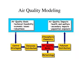
Overview • What are air quality models and why are they useful in regulatory/policy analyses? • What are the key inputs to and outputs from air quality models? • How is international transport treated in air quality modeling? • What are the steps/timing for air quality model applications? • How are air quality models used to project future attainment/nonattainment? • How are air quality models used to provide inputs for calculating benefits? • How are air quality models or tools used to inform control strategy development?
What are Air Quality Models? • Computer programs that contain equations to represent the chemical and physical properties of the atmosphere in relation to air pollutants • In general……. • Models are driven by meteorology and emissions inputs • Models treat the chemical formation and transformation and the dispersion, transport and removal of pollutants • Models output pollutant concentrations and deposition at hourly time steps within grid cells within a user-specified modeling domain (i.e. the area modeled)
Evolution of Air Quality Models • 1st-generation AQM (1970s - 1980s) • Dispersion Models (e.g., Gaussian Plume Models) • Photochemical Box Models (e.g. OZIP/EKMA) • 2nd-generation AQM (1980s - 1990s) • Photochemical grid models (e.g., UAM, RADM) • 3rd-generation AQM (1990s - 2000s) • Community-Based “One-Atmosphere” Modeling System (e.g., CMAQ, CAMx)
Physical Configuration of Grid-based Photochemical Air Quality Models
Integrated Ozone & PM Air Quality Modeling Mobile Sources Ozone NOx, VOC, PM (Cars, trucks, planes, boats, etc.) PM Industrial Sources Chemistry Meteorology NOx, VOC, SOx, PM Visibility (Power plants, refineries/ chemical plants, etc.) Atmospheric Deposition Area Sources NOx, VOC, PM (Residential, farming commercial, biogenic, etc.)
Why are Models useful for Regulatory/ Policy Analyses? • Models provide (the only) means of estimating changes in air quality expected to result from changes in emissions and other environmental conditions (e.g., climate and land-use) • Example uses of air quality models.... • Provide basis or legal justification for Agency action, e.g., OTAQ rules, NOx SIP Call, and CAIR. • Support NAAQS RIAs by helping to identify “cost-effective” control measures for illustrative demonstration of achieving revised standard(s) • Estimate contributions from various sources to air quality problems, e.g., CAIR, designations, and future multi-pollutant sector work • Demonstrate attainment of NAAQS based on controls to be implemented by state/local agencies as part of State Implementation Plans (SIPs)
Air Quality Modeling Platform • Air quality models are typically applied as part of a “Modeling Platform” • Structured system of connected modeling-related tools and data that provide a consistent and transparent basis for assessing the air quality response to changes in emissions and/or meteorology
Key Components of 2002-Based Modeling Platform • 2002 Emissions – mostly from the 2002 National Emissions Inventory (NEI) • 2002 Meteorology from simulations of the PSU Mesoscale Meteorological Model (MM-5) • International Transport (details on slide 15) • Emissions Models, Tools, Projections and Ancillary Data (more on this in a later session) • Air quality Models • Photochemical models: CMAQ & CAMx
2002 Platform Modeling Domains 36 x 36 km Continental US Domain 12 x 12 km Eastern US and Western US Domains 36km Domain Boundary 12km West Domain Boundary 12km East Domain Boundary
What are the Key Inputs to and Outputs from Air Quality Models?
What are the Key Model Inputs? • Emissions inventory • Anthropogenic emissions of NO/NO2, SO2, VOC species, PM species, NH3, and CO • Biogenic VOC species and NO • Meteorology • Winds, temperature, humidity, clouds, precipitation, vertical mixing, etc. • Boundary Conditions • Pollutant concentrations at the domain boundaries which reflect transport from outside the region modeled
What are the Key Model Outputs? • Concentrations of O3 and PM2.5 species • Gridded fields used as inputs to BenMap for calculating health benefits of control strategies • Projected O3 and PM2.5 design values by monitoring site • Used for determining future attainment and residual nonattainment • We now have projections for all monitored counties in the continental US • Projected visibility at IMPROVE sites in Class I Areas • Deposition of pollutants species…e.g., nitrogen and sulfur • Gridded fields which can be converted to Hydrologic Unit Codes (HUC) corresponding to watersheds
How is International Transport Treated in Air Quality Modeling? • Estimates of international transport are obtained from a global chemistry model • GEOSChem – Global chemistry transport model developed at Harvard Univ. • Concentration outputs from the 2002 annual simulation of GEOSChem were provided via the Intercontinental transport and Climatic effects on Air Pollutants (ICAP) project • Domain covers entire globe up to the Stratosphere
What are the Steps/Timing for Air Quality Model Applications?
Air Quality Modeling Process Base Year EI Future Projections Meteorology International Transport Met Pre-Processors Initial/Boundary Concentrations Pre-Processors EMF, SMOKE & Ancillary Files EI Summaries Air Quality Models Raw Outputs Data Archives* Ambient Data Post-Processing Data Fields / Evaluation / Projections / Reports
Timing for Annual Air Quality Model Applications? • Emissions Inventories • Develop new Base Year Inventory ~ several years • Develop Future Base Projections ~ 3 to 6 months • Develop Control Strategies ~ 2 to 3 months • Process Emissions for Input to AQ Model • New Base Year ~ 3 to 6 months and Future Base Case ~ 1 to 2 months • Control Strategies ~ 1 to 2 weeks
Timing for Annual Air Quality Model Applications? • Meteorology – done once • Run meteorological model (e.g., MM5) ~ 3 months + • Process Met for Input to AQ Model ~ 3 weeks • International Transport – done once • Run GEOSChem ~ 4 to 6 weeks • Process Outputs for Input to AQ Model ~ 2 weeks • Air Quality Model Simulations (CMAQ) • Run model for 12 km grid resolution, nationwide ~ 2 weeks • Extractions and post-processing to create products ~ 1 to 2 weeks
How are Air Quality Models used in Regulatory Assessments? • Project future nonattainment/attainment status of areas • Provide inputs for calculating benefits • To inform control strategy development
How are AQ Models used to Project Future Attainment/ Nonattainment? • We use model estimates in a “relative” sense • Premise: models are better at predicting relative changes in concentrations than absolute concentrations • Relative Response Factors (RRF) are calculated by taking the ratio of the model’s future to current predictions of ozone or PM2.5 species • RRFs are calculated for ozone and for each component of PM2.5 and regional haze • Calculation is performed for the location of each ozone and PM2.5 (FRM) monitoring site • For each site, Future DV = Base DV times RRF • Projected ozone and PM2.5 concentrations are, thereby, “tied” to ambient measurements which provides a more robust and scientifically credible future projection of air quality.
Example: Current and 2020 Projected 8-Hour Ozone “Current” Ozone Levels: Average of 8-Hour Ozone Design Values (2000-02, 2001-03, 2002-04) 2020 Base Case Projected 8-Hour Ozone Design Values Model RRF
How are Air Quality Models used to provide Inputs for Calculating Benefits? • Models are typically run for a future base case or baseline scenario along with one or more control strategies • Outputs from the future base case/baseline and control strategy scenarios are provided as gridded concentrations for input to BenMap
Elements of a Benefits Analysis Establish Baseline Conditions (Emissions, Air Quality, Health) Role of Air Quality Models Estimate Expected Reductions in Pollutant Emissions Model Changes in Ambient Concentrations of Ozone and PM Estimate Expected Changes in Human Health Outcomes (Health Impact Analysis) Estimate Expected Changes in Human Health Outcomes (Health Impact Analysis) Estimate Monetary Value of Health Impacts Estimate Monetary Value of Changes in Health Impacts
How are Air Quality Models or Tools used to Inform Control Strategy Development? • Future Base Case/Baseline Modeling • results indicate the location, magnitude, and extent of nonattainment after application of expected control programs • Emissions Sensitivity Modeling • indicates on how air quality may respond to additional controls on one or more pollutants • Source Apportionment/Tagging and “Zero-out” Modeling • useful for estimating the contribution to pollutant concentrations of individual pollutants and sources (or groups of sources)
Overview of Sensitivity Modeling for O3 NAAQS Extrapolated Cost Analysis
Emissions Sensitivity Modeling to Support O3 NAAQS Extrapolated Cost Analysis • Background • The final ozone NAAQS RIA will require an estimate of the full costs of attaining a new ozone standard • The RIA control scenario, which includes all known control measures, is unlikely to result in attainment over all U.S. locations • Thus, we need an estimate of the amount of additional emissions reductions that would yield attainment • The "impact ratio“ approach used for the Proposal RIA contained large uncertainty when applied to individual areas • We are conducting Emissions Sensitivity Modeling to provide more information about the: • nonlinear response of ozone to emissions changes • geographic variation in ozone response • impacts of local versus upwind emissions reductions • relationship between NOx and VOC controls in various areas • Sensitivity modeling will be based off the 2020 070 hypothetical control case emissions
Phase 1: Focus on 4 Key Nonattainment Areas • Emissions Scenarios • Three across-the-board reductions (30, 60, 90%) • Two sets of runs: NOx only, NOx + VOC • Twelve scenarios in total • Four areas: California, Houston, western Lake Michigan, & Northeast Corridor • These areas exceed 80 ppb in the 2020 Base Case, and as such they are expected to have the greatest chance of needing additional controls beyond the RIA control scenario. • Emissions reductions will be applied within 200 km for NOx and 100 km for VOC from each of these four areas • Results will be interpolated to estimate the additional amount of emissions reductions needed for attainment
Phase 2: Impacts of Emissions Reductions in Upwind Areas • Apply emissions reductions in all areas outside the Phase 1 areas with ozone >70 ppb, after application of the RIA control scenario • Single across-the-board reduction will be modeled (30%) • Two sets of runs: NOx only, NOx + VOC • Results will be used to... • develop emissions reduction targets for areas outside the four most problematic areas, and • Modify the local extrapolated tons estimates in the four regions to consider ozone reductions coming from upwind areas