Download
1 / 14
140 likes | 293 Views
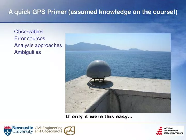
A quick GPS Primer (assumed knowledge on the course!). Observables Error sources Analysis approaches Ambiguities. If only it were this easy…. Review of GPS positioning. Dealing with errors Clock errors (review) Ionosphere (review) Troposphere (part review) Earth body deformations (new)

E N D
A quick GPS Primer (assumed knowledge on the course!) • Observables • Error sources • Analysis approaches • Ambiguities If only it were this easy…
Review of GPS positioning • Dealing with errors • Clock errors (review) • Ionosphere (review) • Troposphere (part review) • Earth body deformations (new) • Orbit errors (new) Orbit Error Clock Error Epsilon (SA) Dither (SA) Ionospheric refraction Tropospheric refraction Receiver Noise Multipath Clock Error
GPS Undifferenced observable A somewhat simplified view, but all these need to be dealt with (at least) for precise GPS geodesy Carrier phase ambiguity Tropospheric Delay True range Satellite j Includes Multipath Observed range Receiver and Satellite clock errors (multiplied by speed of light) Ionospheric Delay Station A
Dealing with clock errors • Undifferenced observable • Estimate both receiver and satellite clocks • Precise Point Positioning – Fix prior satellite clocks and estimate only receiver clocks • Parameter hungry • Double-differenced observable • Undifferenced observations to two satellites at two stations • Form two between-station differences and then double-difference: • Common clock terms difference Satellite j Satellite k Station B Station A
Dealing with orbit errors • These days somewhat easy • Use the IGS final orbits (precise to 2-5cm) • Use Rapid or Ultra-rapid if quick turnaround needed (precise to ~5cm) • Probably no reason to use the broadcast orbits (precise to ~0.5-2m) • In practice • Need orbits from adjacent days when processing against the day boundary • Orbit errors are rarely an error source when using IGS products (main exception is pre-IGS data – earlier than 1994)
Dealing with the Tropospheric Delay (I) • Total delay • ~2.3m at zenith, greater at horizon • Elevation angle dependency may be relatively well modelled with a mapping function (M) for each of two tropospheric components • Two components • Hydrostatic – could be well modelled with accurate pressure • Wet – not well modelled and must be parameterised • Over very short (<<10km) and small elevation difference (<100-200m) baselines, effect cancels in double-difference • General approach • Model hydrostatic with standard pressure or (more accurate) use ECMWF or station met data • Parameterise zenith wet delay (Twet), which also absorbs any residual Thydro , once per 1-2 h (static) or every epoch (kinematic)
Dealing with the Tropospheric Delay (II) • Troposphere is not azimuthally uniform • Horizontal gradients are common, particularly N-S • Highest precision static processing will further estimate horizontal gradient terms • 1-2 for each E-W and N-S per day common • In kinematic analysis, steps in estimated tropospheric zenith delay suggest likely wrong ambiguity fixed and hence quality control
Dealing with Ionospheric Delay (I) • Different frequency signals (in L-band) delayed by different amounts through Ionosphere • Dual frequency GPS receivers allow 99.9% for effect to be removed • Higher order terms may be important for most precise geodetic work • Use a linear combination of L1 and L2 measurements to form new measurement ionosphere free combination for carrier (LC or alternatively L3) • Where are frequency of the L1 and L2 carrier phase signals
Dealing with Ionospheric Delay (II) • Differencing and re-arranging cancels I term • Ionosphere-free phase Linear Combination LC is defined: • Note: • Ambiguity terms are no longer integers – ambiguity fixing is not an option with LC • Noise (“other errors”) is scaled up • General approach • Adopt LC for baselines >~10km • Fix ambiguities, where possible, using a different linear combination (e.g., wide-lane) then final solution using LC, holding ambiguities fixed
Matrix Form • Static case – solving for parameters x A x = b + V Obs1 1-4hrs Obsn
Multipath • Generally dealt with through • Stochastic model by assumption of elevation-dependence and down-weighting lower elevation observations (GAMIT examines the residuals and allows iterative reweighting on a station-by-station basis) • Assuming to “average toward zero” over 24h sessions • Possibly a blind spot in GPS geodesy today
Ambiguity Fixing • Ambiguity for each satellite pass and all cycle slips thereafter • Dozens of ambiguity terms for a 24 h period • Ambiguity fixing process is essentially a series of statistical tests • Can each ambiguity be confidently (given it’s uncertainty) be fixed to an integer? • Iteration required, since uncertainties will change (normally reduce) as ambiguities are fixed and removed from the least squares parameters set • Essential for kinematic (or stabilisation of real-valued estimates in, e.g., Kalman Filter such as in Track) • Not always possible to fix all ambiguities • Less impact for static • Largest effect (normally <10mm) in E, then N & U (see Blewitt, 1989) • Can change the way systematic errors propagate
Double Difference vs PPP • Similar precision possible in 24 h solutions • Software • Few software do geodetic PPP (GIPSY mainly) • GAMIT/Track are Double Difference • PPP is requires extra care • modelling geophysical phenomena (e.g., ocean tide loading displacements) which may be (partially) differenced in relative analysis • orbit/clock errors (some periodic) map 1:1 into positioning • Kinematic PPP requires longer periods of data – ambiguity fixing is not possible without a double difference second step • DD is more precise when short-baseline relative motion is all that is required (e.g., glacier monitoring), but depends on base station
Further Reading • Reference Texts • Hofmann-Wellenhof, B., H. Lichtenegger, and J. Collins. 2001. Global Positioning System: theory and practice, Springer, Wien, 382 pp. • Leick, A. 2004. GPS Satellite Surveying, John Wiley & Sons, New York, 435 pp. • Review Paper • Segall, P., and J.L. Davis. 1997. GPS applications for geodynamics and earthquake studies, Annual Review of Earth Planet Science, 25, 301-336