Download
1 / 47
470 likes | 662 Views
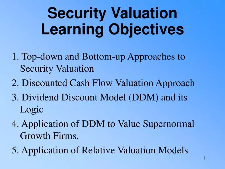
Security Valuation Learning Objectives. 1. Top-down and Bottom-up Approaches to Security Valuation 2. Discounted Cash Flow Valuation Approach 3. Dividend Discount Model (DDM) and its Logic 4. Application of DDM to Value Supernormal Growth Firms. 5. Application of Relative Valuation Models.

E N D
Security ValuationLearning Objectives 1. Top-down and Bottom-up Approaches to Security Valuation 2. Discounted Cash Flow Valuation Approach 3. Dividend Discount Model (DDM) and its Logic 4. Application of DDM to Value Supernormal Growth Firms. 5. Application of Relative Valuation Models
The Investment Decision Process • Determine the required rate of return • Evaluate the investment to determine if its market price is consistent with your required rate of return • Estimate the value based on expected cash flows and your required rate of return • Compare this intrinsic value to the market price • If Intrinsic Value > Market Price, Buy • If Intrinsic Value < Market Price, Don’t Buy
Valuation Process • Two approaches • 1. Top-down, three-step approach • 2. Bottom-up, stock valuation, stock picking approach • The difference between the two approaches is the perceived importance of economic and industry influence on individual firms and stocks
Top-down overview of the valuation process Industry Analysis Structure, supply-demand relationships, quality and cost elements, gov't. regulation, financial norms and standards, et. cetera Economic Analysis Business cycles, government policy, indicators, trade, public attitudes, legislation, inflation, GDP growth, ect. Company Analysis Forecasts, balance sheet--income statement analysis, flow-of-funds analysis, accounting policy and footnotes, management,research, return, risk` GE Other stocks GM, Xerox, Caterpillar, 3M, Merck, Motorola, Delta, Intel. Portfolio management Portfolio Assets
Does the Three-Step Process Work? • An analysis of the relationship between rates of return for the aggregate stock market, alternative industries, and individual stocks showed that most of the changes in rates of return for individual stock could be explained by changes in the rates of return for the aggregate stock market and the stock’s industry
Theory of Valuation • The value of an asset is the present value of its expected returns • To convert this stream of returns to a value for the security, you must discount this stream at your required rate of return • This requires estimates of: • The stream of expected returns, and • The required rate of return on the investment
Stream of Expected Returns • Form of returns • Earnings • Cash flows • Dividends • Interest payments • Capital gains (increases in value) • Time pattern and growth rate of returns
Required Rate of Return • Determined by • 1. Economy’s risk-free rate of return, plus • 2. Expected rate of inflation during the holding period, plus • 3. Risk premium determined by the uncertainty of returns
Valuation Approaches Two Approaches to Equity Valuation Discounted Cash Flow Techniques Relative Valuation Techniques • Price/Earnings Ratio (P/E) • Price/Cash flow ratio (P/CF) • Price/Book Value Ratio (P/BV) • Price/Sales Ratio (P/S) • Present Value of Dividends (DDM) • Present Value of Operating Cash Flow • Present Value of Free Cash Flow
Why and When to Use the Discounted Cash Flow Valuation Approach • The measure of cash flow used • Dividends • Cost of equity as the discount rate • Operating cash flow • Weighted Average Cost of Capital (WACC) • Free cash flow to equity • Cost of equity • Dependent on growth rates and discount rate
Why and When to Use the Relative Valuation Techniques • Provides information about how the market is currently valuing stocks • aggregate market • alternative industries • individual stocks within industries • No guidance as to whether valuations are appropriate • best used when have comparable entities • aggregate market is not at a valuation extreme
Discounted Cash-Flow Valuation Techniques Where: Vj = value of stock j n = life of the asset CFt = cash flow in period t k = the discount rate that is equal to the investor’s required rate of return for asset j, which is determined by the uncertainty (risk) of the stock’s cash flows
The Dividend Discount Model (DDM)-Infinite Holding Period The value of a share of common stock is the present value of all future dividends Where: Vj = value of common stock j Dt = dividend during time period t k = required rate of return on stock j
The Dividend Discount Model (DDM)-Finite Holding Period If the stock is not held for an infinite period, a sale at the end of year 2 would imply: Selling price at the end of year two is the value of all remaining dividend payments, which is simply an extension of the original equation
The Dividend Discount Model (DDM)-Constant Growth Rate Infinite period model assumes a constant growth rate for estimating future dividends Where: Vj = value of stock j D0 = dividend payment in the current period g = the constant growth rate of dividends k = required rate of return on stock j n = the number of periods, which we assume to be infinite
The Dividend Discount Model (DDM)-Constant Growth Rate Infinite period model can be reduced to: Where D1 is the expected dividend, defined as D1= D0 (1+g) 1. Estimate the required rate of return (k) 2. Estimate the dividend growth rate (g)
The Dividend Discount Model (DDM)-Constant Growth Rate Assumptions of DDM: 1. Dividends grow at a constant rate 2. The constant growth rate will continue for an infinite period 3. The required rate of return (k) is greater than the infinite growth rate (g)
Required Rate of Return (k) Three factors influence an investor’s required rate of return: • The economy’s real risk-free rate (RRFR) • The expected rate of inflation (I) • A risk premium (RP) • How to estimate k: K= Rf + (Rm – Rf) K= Bond yield+ERP
Expected Growth Rate of DividendsROE Based • Determined by • the growth of earnings • the proportion of earnings paid in dividends • In the short run, dividends can grow at a different rate than earnings due to changes in the payout ratio • Earnings growth is also affected by compounding of earnings retention g = (Retention Rate) x (Return on Equity) = RR x ROE
Estimating Growth Based on History • Historical growth rates of sales, earnings, cash flow, and dividends • Three techniques 1. arithmetic or geometric average of annual percentage changes 2. linear regression models 3. long-linear regression models • All three use time-series plot of data
How to Calculate g Historical ROE and Payout Year Dividend g = (1-Payout) x ROE • $1.38 = (1 - .50) x .16 = 8% • 1.49 • 1.67 Average of two methods = 8% • 1.75 g = 8%
Infinite Period DDM and Growth Companies Growth companies have opportunities to earn return on investments greater than their required rates of return To exploit these opportunities, these firms generally retain a high percentage of earnings for reinvestment, and their earnings grow faster than those of a typical firm This is inconsistent with the infinite period DDM assumptions
Valuation with Supernormal Growth Example: The last dividend paid (D0) was $2.00. The required rate of return is 14 percent. The dividends are expected to grow at the following rates. What is the value of this stock? Year dividend 1-3: 25% 4-6: 20% 7-9: 15% 10 on: 9%
Computation of Value for Stock of Company with Supernormal Growth
Operating Cash Flow Model • Derive the value of the total firm by discounting the total operating cash flows prior to the payment of interest to the debt-holders • Then subtract the value of debt to arrive at an estimate of the value of the equity
Operating Cash Flow Model Where: Vj = value of firm j n = number of periods assumed to be infinite OCFt = the firms operating cash flow in period t WACC = firm j’s weighted average cost of capital
Operating Cash Flow Model Similar to DDM, this model can be used to estimate an infinite period Where growth has matured to a stable rate, the adaptation is Where: OCF1=operating cash flow in period 1 gOCF = long-term constant growth of operating free cash flow
Operating Cash Flow Model • Assuming several different rates of growth for OCF, these estimates can be divided into stages as with the supernormal dividend growth model • Estimate the rate of growth and the duration of growth for each period
Present Value of Free Cash Flows to Equity • “Free” cash flows to equity are derived after operating cash flows have been adjusted for debt payments (interest and principle) • The discount rate used is the firm’s cost of equity (k) rather than WACC
Present Value of Free Cash Flows to Equity Where: Vj = Value of the stock of firm j n = number of periods assumed to be infinite FCFt = the firm’s free cash flow in period t K j =the cost of equity
Free Cash Flow to Equity Model FCFE = NI + Depreciation – Capital Expenditure - Working Capital – Principal Repayment + New Debt Issues. If capital expenditures and working capital is expected to be financed at the target debt ratio () and principal repayment are made from new debt issues, FCFE can be written as: FCFE = NI + (1- ) (Capital Expenditure - Depreciation) + (1- )Working Capital.
Free Cash Flow to Equity Model FCF is a measure of what firm can payout as dividend. Dividend can be greater than or less than FCF and is influenced by: • Desire for stability • Future Investment Needs • Signaling Affect. P0 = EFCE ; All assumptions about dividend (K – g) valuation model apply.
Relative Valuation Techniques • Value can be determined by comparing to similar stocks based on relative ratios • Relevant variables include: • Price/earnings • Cash flow • Book value • Sales • The most popular relative valuation technique is based on price to earnings
Earnings Multiplier Model The infinite-period dividend discount model indicates the variables that should determine the value of the P/E ratio Dividing both sides by expected earnings during the next 12 months (E1)
Earnings Multiplier Model As an example, assume: • Dividend payout = 50% • Required return = 12% • Expected growth = 8% • D/E = .50; k = .12; g=.08
Earnings Multiplier Model A small change in either or both k or g will have a large impact on the multiplier D/E = .50; k=.13; g=.08 P/E = 10 D/E = .50; k=.12; g=.09 P/E = 16.7 D/E = .50; k=.11; g=.09 P/E = 25
How to Estimate EPS Estimated EPS = Net Income # Shares Outstanding • EPS can also be derived: • EPS = ROE * Book value per share • EPS = NI * E = NI E Shares Shares Where ROE= Profit Margin * Total Asset Turnover * Equity Multiplier
Earnings Multiplier Model Given current earnings of $2.00 and growth of 9% You would expect E1 to be $2.18 D/E = .50; k=.12; g=.09 P/E = 16.7 V = 16.7 x $2.18 = $36.41 Compare this estimated value to market price to decide if you should invest in it
The Price-Sales Ratio • Strong, consistent growth rate is a requirement of a growth company • Sales is subject to less manipulation than other financial data
The Price-Sales Ratio • Match the stock price with recent annual sales, or future sales per share • This ratio varies dramatically by industry • Profit margins also vary by industry • Relative comparisons using P/S ratio should be between firms in similar industries • Average stock price should encompass a long lime period
The Price-Sales Model • Price-to-Sales Model (10 year Average Price Ratios are assumed) • Average Price/Average Sales Per Share • $19.41/14.55=1.33 Price to sales ratio • Vt = P/S ratio*Estimated SPS(t+1) =1.33*$24.65=$32.78
The Price-Cash Flow Ratio • Companies can manipulate earnings • Cash-flow is less prone to manipulation • Cash-flow is important for fundamental valuation and in credit analysis • Price-to-Cash Flow Model • Average Price/Average Cash Flow Per Share • $19.41/1.37=14.17 Cash flow per share ratio • Vt = P/CF*Estimated CFPS (t+1) • Vt = 14.17 * $2.41 = $34.15
The Price-Book Value Ratio Price-to-Book Value Model • Average Price/Average book value per share • $19.41/6.01=3.23 price to book value ratio • Vt = P/BV*Estimated BVPS(t+1) • Vt = 3.23* $10.5 = $33.91
The Price-Book Value Ratio Widely used to measure bank values (most bank assets are liquid (bonds and commercial loans) Fama and French study indicated inverse relationship between P/BV ratios and excess return for a cross section of stocks
The Price-Book Value Model • Price to Book Value Ratio • 1. Po= DPS1 (K-g) *where DPS1=EPS(1+g)*payout ratio • 2. Po= EPSo * Payout * (1+g) (K-g) - where EPS=equity/#shares * NI/equity=BV*ROE • 3. Po= BVo * ROE * Payout * (1+g) (K-g)
Investment Valuation Models • 4. Po = PBV= ROE * Payout * (1+g) BVo (K-g) - i. if ROE depends on expected earnings, or - ii. If payout ratio remains constant 4 becomes 5 • 5. P0 = PBV = ROE * Payout BVo (K-g) -The relationship of: - PBV increase ROE increase - PBV increase Payout increase - PBV increase g increase - PBV decrease K increase
Investment Valuation Models • Formula can be simplified g = ROE (1-payout) ROE*Payout = ROE - g PBV=(ROE-g) / (k-g) Implications: • A) ROE>kP>BV; ROE<kP<BV; ROE=kP=BV • B) PBV decreases if k increases. • C) Larger (R-k) greater PBV