Download
1 / 42
420 likes | 652 Views
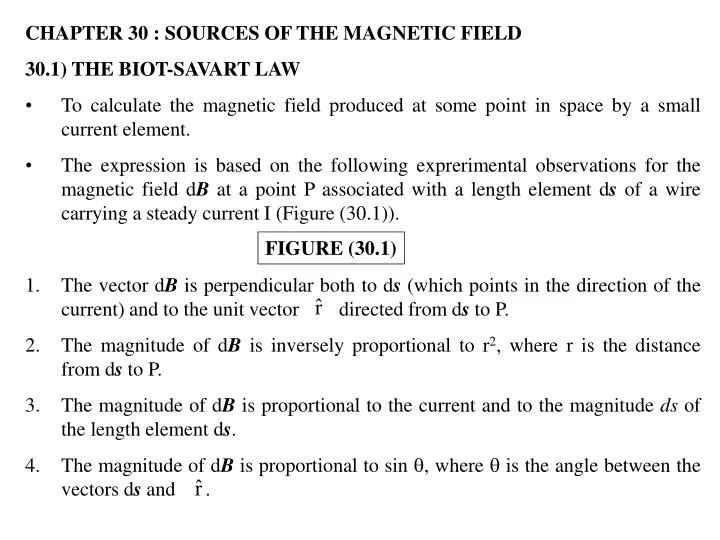
CHAPTER 30 : SOURCES OF THE MAGNETIC FIELD 30.1) THE BIOT-SAVART LAW To calculate the magnetic field produced at some point in space by a small current element.

E N D
CHAPTER 30 : SOURCES OF THE MAGNETIC FIELD • 30.1) THE BIOT-SAVART LAW • To calculate the magnetic field produced at some point in space by a small current element. • The expression is based on the following exprerimental observations for the magnetic field dB at a point P associated with a length element ds of a wire carrying a steady current I (Figure (30.1)). • The vector dB is perpendicular both to ds (which points in the direction of the current) and to the unit vector directed from ds to P. • The magnitude of dB is inversely proportional to r2, where r is the distance from ds to P. • The magnitude of dB is proportional to the current and to the magnitude ds of the length element ds. • The magnitude of dB is proportional to sin , where is the angle between the vectors ds and . FIGURE (30.1)
These observations are summarized in the mathematical formula known today as the Biot-Savart Law : • o is a constant called the permeability of free space : • Notes: The field dB in Equation (30.1) is the field created by the current in only a small length element ds of the conductor. • To find the total magnetic field B created at some point by a current of finite size, we must sum up contributions from all current elements Ids that make up the current. • Evaluate B by integrating Equation (30.1) : (30.1) (30.2) (30.3) where the integral is taken over the entire current distribution.
Similarity between magnetic field and electric field • The current element – produces a magnetic field; • A point charge – produces an electric field. • The magnitude of the magnetic field varies as the inverse square of the distance from the current element. • The magnitude of the electric field is due to the distance from the point charge. • Differences between magnetic field and electric field • Direction of the field • The magnetic field created by a current element is perpendicular to both the length elemetn ds and the unit vector (Equation (30.1)). • The electric field created by a point charge is radial. • Source of the field • The magnetic field is established by an isolated current element. • The electric field is established by an isolated electric charge.
If the conductor lies in the plane of the page (Figure (30.1)), dB points out of the page at P and into the page at P’ (Difference (1)). • The Biot-Savart Law gives the magnetic field of an isolated current element at some point, but such an esolated current element cannot exist the way an esolated electric charge can (Difference (2)). • A current element must be part of an extended current distribution because we must have a complete circuit in order for charges to flow. • Thus, the Biot-Savart law is only the first step in a calculation of a magnetic field; it must be followed by an integration over the current distribution. • Example (30.1): Magnetic Field Surrounding a Thin Straight Conductor • Consider a thin, straight wire carrying a constant current I and placed along the x-axis as shown in Figure (30.2). Determine the magnitude and direction of the magnetic field at point P due to this current. FIGURE (30.2)
Solution • From the Biot-Savart Law, we expect that the magnitude of the field is proportional to the current in the wire and decreases as the distance a from the wire to point P increases. • We start by considering a length element ds located a distance r from P. • The direction of the magnetic field at point P due to the current in this element is out of the page because is out of the page. • In fact, since all of the current elements Ids lie in the plane of the page, they all produce a magnetic field directed out of the page at point P. • Thus, we have the direction of the magnetic field at point P, and we need only find the magnitude. • Taking the origin at O and letting point P be along the positive y axis, with k being a unit vector pointing out of the page, we see that • Where, from Chapter 3, represents the magnitude of .
Solution (continue) • Because is a unit vector, the unit of the cross product is simply the unit of ds, which is length. • Substitution into Equation (30.1) gives : • Because all current elements produce a magnetic field in the k direction, let us restrict our attention to the magnitude of the field due to one current element, which is : • To integrate this expression, we must relate the variable , x and r. • One approach is to express x and r in terms of . • From the geometry in Figure (30.2a), we have : (1) (2)
Solution (continue) • Because tan = a / (-x) from the right triangel in Figure (30.2a) (the negative sign is necessary because ds is located at a negative value of x), we have : • Taking the derivative of this expression gives : • Substitution of Equations (2) and (3) into Equation (1) gives : • an expression in which the only variable is . • We can now obtain the magnitude of the magnetic field at point P by integrating Equation (4) over all elements, subtending angles ranging from 1 to 2 defined in Figure (30.2b) : (3) (4) (30.4)
(30.5) • Solution (continue) • Use this result - to find the magnetic field of any straight current-carrying wire if the geometry, 1, and 2 are known. • Consider the special case of an infinitely long, straight wire. • If we let the wire in Figure (30.2b) become infinitely long, we see that 1 = 0, and 2 = for length elements ranging between positions x = - and x = +. • Because (cos 1 - 2 ) = (cos 0 - cos ) = 2, Equation (30.4) becomes : • Equation (30.4) and (30.5) both show that the magnitude of the magnetic field is proportional to the current and decreases with increasing distance from the wire. • Equation (30.5) has the same mathemetical form as the expression for the magnitude of the electric field due to a long charged wire (see Equation (24.7)).
FIGURE (30.3) • Explaination for Figure (30.3) • Figure (30.3) is a three-dimensional view of the magnetic field surrounding a long, straight current-carrying wire. • Because of the symmetry of the wire, the magnetic field lines are circles concentric with the wire and lie in planes perpendicular to the wire.the magnitude of B is constant on any circle of radius a and is given by Equation (30.5). • A convenient rule for determining the direction of B is to grasp the wire with the right hand, positioning the thumb along the direction of the current. • The four fingers wrap in the direction of the magnetic field.
A’ A R O R C I C’ Example (30.2) : Magnetic Field Due to a Curved Wire Segment Calculate the magnetic field at point O for the current-carrying wire segmetn shown in Figure (30.4). The wire consists of two straight portions and a circular are of radius R, which subtends an angle . The arrowheads on the wire indicate the direction of the current. FIGURE (30.4)
Solution • The magnetic field at O due to the current in the straight segments AA’ and CC’ is zero because ds is parallel to along these paths; this means that • Each length element ds along path AC is at the same distance R from O, and the current in each contributes a field element dB directed into the page at O. • Furthermore, at every point on AC, ds is perpendicular to ; hence, • Using this information and Equation (30.1), we can find the magnitude of the field at O due to the current in an element of length ds : • Because I and R are constants, we can easily integrate this expression over the curved path AC:
Solution (continue) • where we have used the fact that s = R measured in radians. • The direction of B is into the page at O because is into the page for every length element. • Example (30.3) : Magnetic Field on the Axis of a Circular Current Loop • Consider a circular wire loop of radius R located in the yz plane and carrying a steady current I, as shown in Figure (30.5). Calculate the magnetic field at an axial point P a distance x from the center of the loop. (30.6) FIGURE (30.5)
Solution • In this situation, note that every length element ds is perpendicular to the vector at the location of the element. • Thus, for any element, • Furthermore, all length elements around the loop are at the same distance r from P, where r2 = x2 + R2. • Hence, the magnitude of dB due to the current in any length element ds is : • The direction of dB is perpendicular to the plane formed by and ds (Figure (30.5)). • We can resolve this vector into a component dBx along the x axis and a component dBy perpendicular to the x axis. • When the components dBy are summed over all elements around the loop, the resultant component is zero.
Solution (continue) • That is, by symmetry the current in any element on one side of the loop sets up a perpendicular component of dB that cancels the perpendicular component set up by the current through the element diametrically opposite it. • Therefore, the resultant field at P must be along the x axis and we can find it by integrating the components dBx = dB cos . • That is, ,where • and are must take the integral over the entire loop. • Because , x, and R are constants for all elements of the loop and because cos = R / (x2 + R2)1/2, we obtain : (30.7) where (the circumference of the loop)
Solution (continue) • To find the magnetic field at the center of the loop, we set x = 0 in Equation (30.7). • At this special point, therefore, • which is consistent with the result of the exercise in Example (30.2). • It is also interesting to determine the behavior of the magnetic field far from the loop – that is, when x is much greater than R. • In this case, we can neglect the term R2 in the denominator of Equation (30.7) and obtain : • Because the magnitude of the magnetic moment of the loop is defined as the product of current and loop area (see Equation (29.10) : = I( R2 ) for our circular loop – we can express Equation (30.9) as : (at x = 0) (30.8) (30.9) (for x >> R
Solution (continue) • This result is similar in form to the expression for the electric field due to an electric dipole, E = ke (2qa/y3) (See Example (23.6)), where 2qa = p is the electric dipole moment as defined in Equation (26.16). • The pattern of the magnetic field lines for a circular current loop is shown in Figure (30.6a) pg 943. • The field-line pattern is axially symmetric and looks like the pattern around a bar magnet, shown in Figure (30.6c) pg 943. (30.10)
30.2) THE MAGNETIC FORCE BETWEEN TWO PARALLEL CONDUCTORS • Consider two long, straight, parallel wires separated by a distance a and carrying currents I1 and I2 in the same direction (Figure (30.7). • We can determine the force exerted on one wire due to the magnetic field set up by the other wire. • Wire 2, which carries a current I2, creates a magnetic field B2 at the location of wire 1. • The direction of B2 is perpendicular to wire 1, as shown in Figure (30.7) • According to Equation (29.3), the magnetic force on a length of wire 1 is : • Because is perpendicular to B2 in this situation, the magnitude of F1 is F1 = I1 B2 . • Because the magnitude of B2 is given by Equation (30.5), we see that (30.11)
The direction of F1 is toward wire 2 because is in that direction. • If the field set up at wire 2 bywire 1 is calculated, the force F2 acting on wire 2 is found to be equal in magnitude and opposite in direction to F1. • When the currents are in opposite directions (that is, when one of the currents is reversed in Figure (30.7), the forces are reversed and the wires repel each other. • Hence, we find that parallel conductors carrying currents in the same direction attract each other, and parallel conductors carrying currents in opposite directions repel each other. • Because the magnitudes of the forces are the same on both wires, we denote the magnitude of the magnetic force between the wires as simply FB. • We can rewrite this magnitude in terms of the force per unit length : • The force between two parallel wires is used to define the ampere as follows : (30.12) When the magnitude of the force per unit length between two long, parallel wires that carry identical currents and are separated by 1m is 2 x 10⁻⁷N/m, the current in each wire is defined to be 1A.
The value 2 x 10⁻⁷N/m is obtained from Equation (30.12) with I1 = I2 = 1A, and a = 1m. • The SI unit of charge, the coulomb, is defined in terms of the ampere : • In deriving Equation (30.11) and (30.12) we assumed that both wires are long compared with their separation distance. • In fact, only one wire needs to be long. • The equations accurately describe the forces exerted on each other by a long wire and a straight parallel wire of limited length When a conductor carries a steady current of 1A, the quantity of charge that flows through a cross-section of the conductor in 1s is 1C.
30.3) AMPERE’S LAW • Compass needles point in the direction of B when place near the current-carrying conductor. • Refering Figure (30.8) pg. 945 – several compass needles are palced in a horizontal plane near a long vertical wire. • When no current is present in the wire, all the needles point in the same direction (that of the Earth’s mangetic field), as expected ((Figure (30.8a)). • When the wire carries a strong, steady current, the needles all deflect in a direction tangent to the circle, (Figure (30.8b)). • The direction of the magnetic field produce by the current in the wire is consistent with the right-hand rule (Figure (30.3)) • When the current is reversed, the needles in Figure (30.8b) also reverse. • The lines of B form circles around the wire, therefore : • The magnitude of B is the same everywhere on a circular path centered on the wire and lying in a plane perpendicular to the wire • By varying the current and distance a from the wire – B is proportional to the current and inversely proportional to the distance from the wire (Eq. (30.5)).
Let us evaluate the product B·ds for a small length element ds on the circular path defined by the compass needles, and sum the products for all elements over the closed circular path. • Along this path, the vectors ds and B are parallel at each point (Figure (30.8b)), so B·ds = Bds. • Furthermore, the magnitude of B is constant on this circle and is given by Equation (30.5). • Therefore, the sum of the products Bds over the closed path, which is equivalent to the line integral of B·ds, is : • where is the circumference of the circular path. • Although this result was calculated for the special case of a circular path surrounding a wire, it holds for a closed path of any shape surrounding a current that exists in an unbroken circuit.
The general case, known as Ampere’s Law, can be stated as follows : • Notes: Ampere’s Law – to calculate the magnetic field of current configurations having a high degree of symmetry. • Example (30.4) : The Magnetic Field Created by a Long Current-Carrying Wire • A long, straight wire of radius R carries a steady current Io that is uniformly distributed through the cross-section of the wire (Figure (30.11)). Calculate the magnetic field a distance r from the center of the wire in the regions and . The line integal of B·ds around any closed path equals oI, where I is the total continuous current passing through any surface bounded by the closed path. (30.13) FIGURE (30.11)
Solution • For the case, we should get the same result we obtained in Example (30.1), in which we applied the Biot-Savart law to the same situation. • Let us choose for our path of integration circle 1 in Figure (30.11). • From symmetry B must be constant in magnitude and parallel to ds at every point on this circle. • Because the total current passing through the plane of the circle is Io, Ampere’s law gives : • which is identical in form to Equation (30.5). (for ) (30.14)
Solution (continue) • Now consider the interior of the wire, wher r < R. • Here the current I passing through the plane of circle 2 is less than the total current Io. • Because the current is uniform over the cross-section of the wire, the fraction of the current enclosed by circle 2 must equal the ratio of the area r2 enclosed by circle 2 to the cross-sectional area R2 of the wire : • Folloeing the same procedure as for circle 1, we apply Ampere’s law to circle 2 : (for r < R) (30.15)
Example (30.5) : The Magnetic Field Created by a Toroid • A device called a toroid (Figure (30.13)) is often used to create an almost uniform magnetic field in some enclosed area. The device consists of a conductiong wire wrapped aroung a ring (a torus) made of a nonconducting material. For a toroid having N closely spaced turns of wire, calculate the magnetic field in the region occupied by the torus, a distance r from the center. • Solution • To calculate this field, we must evaluate over the circle of radius r in Figure (30.13). • By symmetry, we see that the magnitude of the field is constant on this circle and tangent to it, so FIGURE (30.13)
(30.16) • Solution (continue) • Furthermore, note that the circular closed path surrounds N loops of wire, each of which carries a current I. • Therefore, the right side of Equation (30.13) is oNI in this case. • Ampere’s law applied to the circle gives :
Example (30.6) : Magnetic Field Created By an Infinite Current Sheet • So far we have imagined currents through wires of small cross-section. Let us now consider an example in which a current exists in an extended object. A thin, infinitely large sheet lying in the yz plane carries a current of linear current density Js. The current is in the y direction, and Js represents the current per unit length measured along the z-axis. Fing the magnetic field near the sheet. • Solution • This situation brings to mind similar calculations involving Gauss’s law (Ex. (24.8)). • Recall that the electric field due to an infinite sheet of charge does not depend on distance from the sheet. • We might expect a similar result here for the magnetic field. FIGURE (30.14)
To evaluate the line interal in Ampere’s law, let us take a rectangular path through the sheet, (Figure (30.14)).the rectangel has dimensions parallel to the sheet surface. • The net current passsing through the plane of the rectangle is Js . • We apply Ampere’s law over the rectangel and note that the two sides of length w do not contribute to the line integral because the component of B along the direction of these paths is zero. • By symmetery, we can argue that the magnetic field is constant over the sides of lenth because every point on the infinitely large sheet is equaivalent, and hence the field should not vary from point to point. • The only choices of field direction that are reasonable for the symmetry are perpendicular or parallel to the sheet, and a perpendicular field would pass through the current, which is inconsistent with the Biot-Savart law. • Assuming a field that is cosntant magnitude and parallel to the plane of the sheet, we obtain :
Example (30.7) : The Magnetic Force on a Current Segment • Wire 1 in Figure (30.15) is oriented along the y axis and carries a steady current I1. A rectangular loop located to the right of the wire and in the xy plane carries a current I2. Find the magnetic force exerted by wire 1 on the top wire of length b in the loop, labeled “Wire 2” in the figure. • Solution • Consider the force exerted by wire 1 on a small segmetn ds of wire 2 by using Equation (29.4). • This force is given by where I = I2 and B is the magnetic field created by the current in wire 1 at the position of ds. • From ampere’s law, the field at a distance x from wire 1 (see Equation (30.14)) is : FIGURE (30.15)
Solution (continue) • where the unit vector is used to indicate that the field at ds points into the page. • Because wire 2 is along the x axis, ds = dx i, and we find that : • Integrating over the limits x = a to x = a+b gives : • The force points in the positive y direction, as indicated by the unit vector and as shown in Figure (30.15).
Indicating that the field in this space is uniform and strong. • 30.4) THE MAGNETIC FIELD OF A SOLENOID • A solenoid is a long wire wound in the form of a helix. • With this configuration, a uniform magnetic field can be produce in the space surrounded by the turns of wire (= the interior of the solenoid – when the solenoid carries a current). • When the turns are closely spaced, each can be approximated as a circular loop, and the net magnetic field is the vector sum of the fields resulting from all the turns. • Figure (30.16) • Figure (30.16) – shows the magnetic field lines surrounding a loosely wound solenoid. • The field lines in the interior are : • 1. nearly parallel to one another • 2. uniformly distributed • 3. close together, FIGURE (30.16)
The field lines between current elements on two adjacent turns tend to cancel each other because the field vectors from the two elements are in opposite directions. • The field at exterior points such as P is weak because the field due to current elements on the right-hand portion of a turn tends to cancel the field due to current elements on the left-hand portion. • If the turns are closely spaced and the solenoid is of finite length, the magnetic filed lines are as shown in Figure (30.17a), pg. 950. • This field lines distribution is similar to that surrounding a bar magnet (Figure (30.17b), pg. 950). • One end of the solenoid behaves like the north pole of a magnet, and the opposite end behaves like the south pole. • As the length of the solenoid increases, the interior field becomes more uniform and the exterior field becomes weaker. FIGURE (30.17)
2 1 3 4 • An ideal solenoid is approached when the turns are closely spaced and the length is much greater than the radius of the turns. • In this case, the external field is zero, and the interior field is uniform over a great volume. • Ampere’s law – to obtain an expression for the interior magnetic field in an ideal solenoid. • Figure (30.18) – shows a longitudinal cross-section of part of such a solenoid carrying a current I. FIGURE (30.18)
Because the solenoid is ideal, B in the interior space is uniform and parallel to the axis, and B in the exterior space is zero. • Consider the rectangular path of length and width (Figure (30.18)). • Apply Ampere’s Law to this path by evaluating the integral of B.ds over each side of the rectangle. • The contribution along side 3 is zero because B = 0 in this region. • The contributions from sides 2 and 4 are both zero because B is perpendicular to ds along these paths. • Side 1 gives a contribution to the integral because along this path B is uniform and parallel to ds. • The integral over the closed rectangular path is therefore: • The right side of Ampere’s law inbolves the total current passing through the area bounded by the path of integration.
In this case, the total current through the rectangular path equals the current through each turn multiplied by the number of turns. • If N is the number of turns in the length , the total current through the rectangle is NI. • Therefore, Ampere’s law applied to this path gives : • where n = N / is the number of turns per unit length. • By reconsidering the magnetic field of a toroid (Example (30.5)) – we can also obtain Equation (30.17). • If the radius r of the torus in Figure (30.13), pg. 948, containing N turns is much greater than the toroid’s cross-sectional radius a, a short section of the toroid approximates a solenoid for which n = N / 2r. (30.17) Magnetic field inside a solenoid
Notes : • In this limit, Equation (30.16) agrees with Equation (30.17). • Equation (30.17) is valid only for points near the center (that is, far from the ends) of a very long solenoid. • The field near each end is samaller than the volume given by Equation (30.17). • At the very end of a long solenoid, the magnitude of the field is one-half the magnitude at the center. • 30.5) MAGNETIC FLUX • The flux associated with a magnetic field is defined in a manner similar to that used to define electric flux (Eq. (24.3)). • Consider an element of area dA on an arbitrarily shaped surface, as shown in Figure (30.19). • If the magnetic field at this element is B, the magnetic flux through the elemetn is B.dA, where dA is a vector that is perpendicular to the surface and has a magnitude equal to the area dA.
(30.18) (30.19) • The total magnetic flux B through the surface is : • Consider the special case of a plane of area A in a uniform field B that makes angle with dA. • The magnetic flux through the plane in this case is : Definition of Magnetic Flux FIGURE (30.19)
(a) (b) • If the magnetic field is parallel to the plane, as in Figure (30.20a), then = 90o and the flux is zero. • If the field is perpendicular to the plane, (Figure (30.20b)), then = 0, and the flux is BA (the maximum value). • The unit of flux is the T.m2, which is defined as a weber (Wb); 1Wb = 1 T.m2. FIGURE (30.20)
dr I b r c a Example (30.8): Magnetic Flux Through a Rectangular Loop A rectangular loop of width a and length b is located near a long wire carrying a current I (Figure (30.21)). The distance between the wire and the closest side of the loop is c. the wire is parallel to the long side of the loop. Find the total magnetic flux through the loop due to the current in the wire. FIGURE (30.21)
Solution • Form Equation (30.14), we know that the magnitude of the magnetic field created by the wire at a distance r from the wire is : • The factor 1/r indicates that the field varies over the loop, and Figure (30.21) shows that the field is directed into the page. • Because Bis parallel to dA at anypoint within the loop, the magnetic flux through an area element dA is : • To integrate, we first express the area element (the tan region in Figure (30.21) as dA = bdr). (Because B is not uniform but depends on r, it cannot be removed from the integral)
Because r is now the only variable in the integral, we have : • 30.6) GAUSS’S LAW IN MAGNETISM • Gauss’s Law = the electric flux through a closed surface surrounding a net charge is proportional to that charge. • - In other words, the number of electric field lines leaving the surface depends only on the net charge within it. • - This property is based on the fact that electric field lines originate and terminate on electric charges. • The situation is quite different for magnetic field, which are continuous and form closed loops. • In other words, magnetic field lines do not begin or end at any point – as illustrated by the magnetic field lines of the bar magnet in Figure (30.22).
The net magnetic flux through any closed surface is always zero : (30.20) Gauss’s Law for magnetisim FIGURE (30.22) • For any closed surface, such as the one outlined by the dashed line in Figure (30.22), the number of lines entering the surface equals the number leaving the surface; thus, the net magnetic flux is zero. • In contrast, for a closed surface surrounding one charge of an electric dipole (Figure (30.23)), the net electric flux is not zero. • Gauss’s Law in magnetism states that :