Download
1 / 28
280 likes | 370 Views
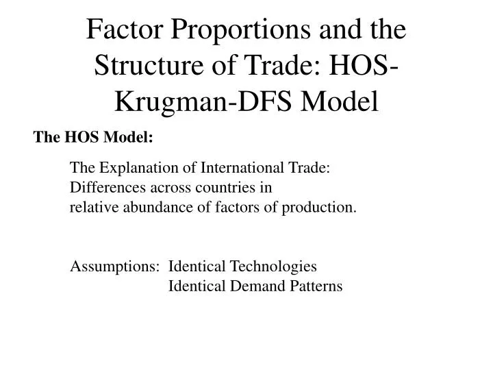
Factor Proportions and the Structure of Trade: HOS-Krugman-DFS Model. The HOS Model:. The Explanation of International Trade: Differences across countries in relative abundance of factors of production. Assumptions: Identical Technologies Identical Demand Patterns. Relative Factor

E N D
Factor Proportions and the Structure of Trade: HOS-Krugman-DFS Model The HOS Model: The Explanation of International Trade: Differences across countries in relative abundance of factors of production. Assumptions: Identical Technologies Identical Demand Patterns
Relative Factor Intensity : Full employment: Y E K constant A B* B L constant D F X C Structural Bias: The Transformation Curve( = ABC) shifts asymmetrically with unbalanced changes in K and L. A Rise in K, with no change in L, leads to an increase(fall) in X (Y)).
AT POINT F 1) Labor is unemployed: W=0. (2) The X-industry is active The Y-industry is inactive. Therefore: AT POINT A 1) Capital is unemployed: R=0. (2) Y-industry is active X-industry is inactive. Therefore:
At Point B Relative Supply
Two Countries: H and F: H is more capital abundant. H’s Relative Supply is biased towards X:
Free Trade and Autarkic Equilibria 3 2 1 2=Free trade 1=autarky in H 3=autarky in F
The Heckscher-Ohlin Proposition #1: Any country will export the good which makes intensive use in its production of relative abundant factor supply.
Income Distribution and International Trade W A Industry X-Line B B’ Industry Y-Line C D R ABC=factor price frontier A rise in (X is capital intensive) will raise R and decrease W.
The Heckscher-Ohlin Proposition #2(dual to Proposition #1): Free trade causes an increase in the factor price of the factor of production which is used intensively in the export industry and a fall in the factor price used intensively in the import competing industry.
Factor Price Equalization: Failures Two ways to generate a failure of FPE: • Assume that factor proportions are sufficiently different that they are outside the FPE set. • Introduce costs to international trade, which could have strong effect on trade volume.
Romalis (AER, March 2004, 94, No.1, 67-97) • Generalizes a Heckscher-Ohlin model of Dornbusch-Fischer-Samuelson framework, and explains trade structure; • Assumes a many-country version of the Heckscher-Ohlin model; • Integrates this with Krugman intra-industry trade; • Allows for transportation costs.
The Model There are 2M countries, M each in the North and South. Southern variables are marked with an asterisk. There are two factors of production: skilled and unskilled labor. The proportion of skilled labor is Northern countries are abundant in skilled labor
Monopolistic Competition = Production of variety i Number of of varieties in industry z Number of countries Sub-utility function Dual Unit cost Fixed cost
Transportation costs Units of a good must be shipped for 1 unit to arrive in any other country
Equilibrium in an industry Solve for the share of world production that each country commands, conditional on relative production costs. Countries with lower costs capture larger market shares. Consumer price Ideal Price index
National income and Spending A constant fraction of income b(z) is spent on industry z
If is low, (1) is the solution;if is high, (2) is the solution (1) (2)
Special Case The Dornbusch-Fischer-Samuelson Model is a special case with no transportation costs Perfect competition
Transport costs The addition of the transport costs leads a stark structure of production and trade: Non-traded goods Produced In South Skill intensity of industry (z) Share of industry Skill-intensive goods Produced In North Non-traded goods Produced In North Unskilled goods produced in south
Producer prices p=factory-gate price domestically; Sold in M-1 markets abroad