Download

1 / 36
360 likes | 570 Views
Background. Over 170 exoplanets known.1Many in multi-planet systems.Most from radial velocity data.As more data is accumulated it will be useful to have an automated procedure, which should:Decide on the number of planets.Give orbital parameters and errors.Decide on whether to include a long-t

E N D
1. Towards an Automated Procedure for the Detection of Planetary Systems in Radial Velocity Surveys Raman Narayan
Advisor: Dr. Debra Fischer
2. Background Over 170 exoplanets known.1
Many in multi-planet systems.
Most from radial velocity data.
As more data is accumulated it will be useful to have an automated procedure, which should:
Decide on the number of planets.
Give orbital parameters and errors.
Decide on whether to include a long-term trend.
Assess the significance of a detection.
3. Overview Radial velocity parameters and equations
Lomb-Scargle Periodogram
Single-planet automated procedure
Multi-planet procedure
Additional multi-planet tools
Discussion and future work
4. Orbital Parameters Orbital period, P
Time of periastron passage, tp
Eccentricity, e
Longitude of periastron, O
Velocity amplitude, K
5. Radial Velocity Equation vr is the component of the star�s velocity along our line of sight.
e and O determine the shape of the periodic signal.
We also include an additive constant representing the cm-velocity of the system.
For multiple planets, assuming no interactions, signals are superimposed.
6. Periodograms Similar to a power spectrum, or discrete data analog of a Fourier transform.
The periodograms used here are closely related to the Lomb-Scargle Periodogram.
A measure of the improvement of fitting a single sinusoid plus a constant to the data over fitting only a constant.
Each peak has a width of ~1/T in frequency space, where T is the time spanned by the data.
Periodogram power z(?) is evaluated for a grid of orbital frequencies, separated here by 1/(4T).
Highest peaks are optimized to increase precision in the corresponding orbital frequency or period.
7. Floating Mean/Trend Periodogram Function of ?2 for a particular orbital frequency.
m = 1 for a floating constant, 2 for a line, 3 for a parabola.
The floating mean/trend can be very important.
8. False Alarm Probability Our measure of the significance of a detection.
Definition: probability that random noise would conspire to give a maximum periodogram power = that due to the planet in question.1
Calculated here using Monte Carlo simulations.
The FAP is the fraction of trials where the max power met or exceeded the power of the peak in question.
�Noise data� used affects interpretation.
Gaussian deviates suggested by assigned errors (used here).
Gaussian deviates with variance equal to that of the data.
Bootstrap method (scrambling data).
In all three we preserve original times and error bars.
9. Example of Periodogram Analysis Sinusoid plus noise.
We add 20 observations at a time; 200 shown at right.
10. For N = 20, 40, 60, 80, 100, 120, 140, 160, 180, 200 observations, left to right, top to bottom.
Vertical line represents correct period.
Horizontal lines for detection thresholds corresponding to FAP�s of F = 0.1 (lower) and F = 0.01 (upper).
Initial decrease in FAP is probably due to increase in number of independent frequencies. Floating-mean Periodograms
11. Analytic FAP Formula z0 = peak power
Ni = # of independent frequencies.
?f = range of frequencies sampled.
Solid line: Monte Carlo.
Dotted line: analytic formula.
Dashed line: analytic formula with no signal.
?�s: highest peak corresponds to correct period.
*�s: highest peak does not correspond to the correct period.
If accuracy is important, we use the Monte Carlo method.
12. Finding the Orbital Parameters for a Single Planet The procedure is explained using a simulated system.
300 observations over 3 years (100 per �season�).
13. 1. Floating-parabola periodogram All peaks within some fraction (we use e-1/2 � 0.607) of the highest peak are considered.
A detection threshold can be used as an additional criteria.
Only one peak qualifies here. It has periodicity P = 39.855 days.
14. 2. Keplerian fit For each qualifying peak, we perform a Keplerian fit which includes a floating parabola.
Levenberg-Marquardt method for non-linear least-squares.
Sinusoid parameters from the periodogram provide input parameters.
15. 3. Long-term trend or not? If there are additional planets it the data with periods longer than a few T, then there may be a long-term trend that cannot be recognized as a Keplerian orbit.
We would like to know whether to keep the parabolic trend, adopt a linear trend, or fit no long-term trend at all.
We perform additional Keplerian fits including a linear trend and no trend.
Fractional changes in ?2 are compared to those from the ?2 � distribution, given some cutoff probability, to determine the order of the trend.
This step could be omitted if one would rather keep a linear or parabolic trend than decide.
In this example we choose to keep a linear trend.
16. 4. Parameter Errors We calculate parameter uncertainties using Monte Carlo Simulations.
Simulated data sets consist of the fitted model plus random noise at the level suggested by the assigned errors (error bars).
Additional noise is added if reduced ?2 > 1.
We generate distributions (see histograms at right) for each parameter and take the standard deviation as the uncertainty in each parameter.
17. Results of Single-planet Example In this case we only have one set of parameters. There will be a set of parameters for each qualifying periodogram peak.
Sometimes ?2 indicates the best solution, other times the correct choice is not clear.
18. Plots of the Results of the Single-planet Example Top panel: fitted Keplerian orbit and linear trend. The dashed line represents the simulated signal.
Bottom panel: phased plot of the fitted model, where the fitted linear trend has been subtracted.
19. Multiple Planets Many of the same techniques used in the single-planet case are still applicable.
We use another simulated data set to demonstrate our procedure.
The procedure will culminate in a multi-Keplerian fit.
This can be computationally expensive.
If we try 4 different values for O for each planet and we are fitting for Npl planets, we will have to minimize ?2 4Npl times.
We must build up sufficient input parameters for the multi-Keplerian fit, so that we will find the global minimum of ?2 .
This may be the greatest challenge.
There will likely be more possible solutions than in the single-planet case.
20. Searching the Residuals We use the same techniques as in the single-planet case.
The residuals are searched for additional planets.
This method is illustrated using the simulated data set shown below.
Same times and errors as in single-planet example.
21. 1. Single-Keplerian fit We evaluate the floating-parabola periodogram and fit a single Keplerian orbit as in the single-planet case.
Don�t decide on trend; we keep a parabola for now.
Peaks higher than both e-1/2 of the highest peak (dashed line) and a detection threshold corresponding to an FAP of F = 0.01 (dotted line) are considered.
The 2 qualifying peaks in this example are marked with asterisks.
22. 2. Search Residuals We begin with the highest peak from the periodogram of the original data.
Obtain residuals by subtracting the previously fitted Keplerian orbit (not subtracting the trend).
Evaluate floating-parabola periodogram of residuals (next slide).
The same criteria as before are used to decide on which peaks to consider (only 1 peak here).
Perform 2-Keplerian fit, including parabolic trend.
Input parameters are provided by the previous single-Keplerian fit, and the periodogram of the residuals.
Obtain residuals of the 2-Keplerian fit (not subtracting the trend).
Evaluate the periodogram of these (second) residuals.
If there are qualifying peaks, repeat from (1.) for 3-planets.
If not, move on to the next peak from the first residuals (the case in this example).
23. 3. Decide on the long term trend. This is done in the same way as in the single-planet case.
Now the ?2 compared are for multi-Keplerian fits.
In this case (cutoff value of 0.05) we choose not to include a trend.
The top panel shows the periodogram of the (first) residuals. The bottom panel shows the fitted model (solid curve) and the simulated model (dashed curve).
The fit would be closer if the a long term trend had been kept.
24. 4. Parameter errors Calculated in the same way as with a single planet.
If one cycles though different values for O this can be very time consuming.
We don�t try multiple guesses for O here.
Histograms are shown at right.
25. 5. Results This automated procedure will usually result a number of models for the system.
We usually choose the one with the lowest ?2 as the �correct� solution, which we assume represents the global minimum of ?2 in parameter space.
Sometimes there will be multiple distinct solutions (in this case there is only one).
26. Additional Tools for Multiple Planets Our automated procedure for multi-planet systems, though successful in many cases, is not always able to find the correct solution.
We discuss two tools that may be used in a more robust analysis of multi-planet systems.
They are demonstrated using the simulated data set shown at right, which contains two planets and no long-term trend.
27. Analysis with Residuals Analysis using our automated routine.
Top: The periodogram of the simulated data and single Keplerian fits.
Bottom: The periodogram of the residuals from the model shown in green, where P � 123 days, and the final solution (solid curve, reduced ?2 = 0.904 ). The residuals from the other model produced no qualifying peaks. The dashed curve represents the simulated signal.
28. 2-dimensional Periodogram Measures the improvement in fitting 2 sinusoids plus a floating constant/trend over fitting a floating constant/trend.
The first periodicity (days) is plotted against the second.
Regions where the power is lowest appear black and those with the most power appear red.
The highest peaks are marked with x�s.
Most useful where there are two planets with similar velocity amplitudes.
Has problems with highly eccentric orbits.
29. Kepler-sine Periodogram Measures the improvement in fitting a Keplerian orbit plus a sinusoid over a fitting a Keplerian orbit.
Takes sinusoid or single-Keplerian parameters x1 as input.
Can be less robust than the 2-d periodogram because of the dependence on input parameters.
The dotted line represents the periodicity from x1 .
30. Results Model 1 is found using both residuals and the 2-d periodogram.
Using residuals alone, we never find Model 2, which is closer to the simulated signal.
The Kepler-sine periodogram gives similar results to the 2-d periodogram in this case.
The weakness in our automated procedure appears to be its dependence on contaminated residuals.
The initial fit corresponding to the ~390 day periodicity deviated greatly from the signal it was supposed to represent.
31. 51 Pegasi First planet found orbiting a Sun-like star in 1995.1
51 Peg b has an orbital period of 4.23 days.2
3 different dewars were used (shown as different colors).
32. Periodograms and Initial Fit The floating-parabola periodogram is evaluated for each dewar.
All have highest peaks at 4.23 days.
A single Keplerian orbit with a parabolic trend is fit for each dewar.
33. Residuals We first subtract the well-known signal of 51 Peg (top panel).
There appears to be a pronounced offset due to the second dewar change.
The constant and trend are subtracted as well (lower panel).
34. Periodograms of the Residuals Floating-parabola periodograms are evaluated before the parabolic trends are subtracted.
The dotted lines, where they appear, correspond to a detection threshold where F = 0.01.
Calculated by Monte Carlo where noise was simulated at the level of the error bars.
The dashed lines represents e-1/2 of the highest peak.
35. Results for Combined Residuals We now treat the residuals, with the trends and constants subtracted, as a single data set.
The floating-mean periodogram is evaluated.
There are several peaks of similar height superimposed on the broad peak at ~17 days.
Detection thresholds corresponding to both �error bar� and �bootstrap� Monte Carlo simulations are shown.
In both cases, the highest peak has an FAP of F < 0.001.
FAP�s may not be reliable for residuals.
A phased plot of the circular orbit corresponding to the highest peak is shown at right.
36. Future Work Incorporate 2-d and Kepler-sine periodograms in automated routines.
Calculating and interpreting the FAP for multi-planet systems.
We calculated the FAP using the residuals in the same way as it was done in the single-planet case with the original data.
Incorporate other techniques that have been used in analyzing radial velocity data.
�Kepler periodograms� (for example, Cumming 2004)
Bayesian techniques (for example, Gregory 2005)
Inclusion of interplanetary interactions.
Necessary for Gliese 876 (Rivera et al. 2005)