Download
1 / 19
260 likes | 561 Views
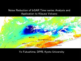
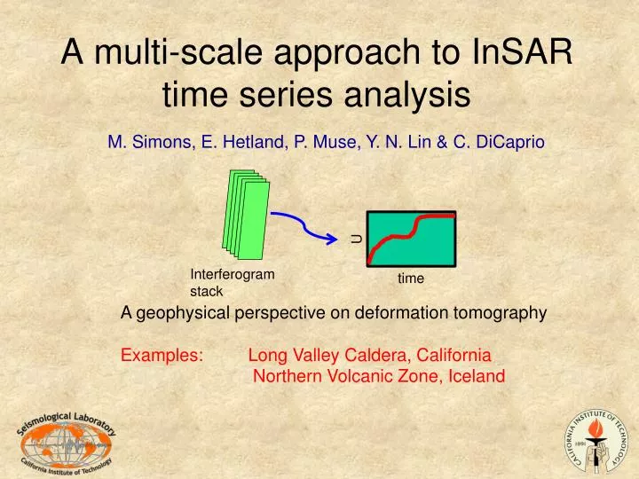
M. Simons, E. Hetland, P. Muse, Y. N. Lin & C. DiCaprio. A multi-scale approach to InSAR time series analysis. Interferogram stack. A geophysical perspective on deformation tomography Examples: Long Valley Caldera, California Northern Volcanic Zone, Iceland. U. time.

E N D
M. Simons, E. Hetland, P. Muse, Y. N. Lin & C. DiCaprio A multi-scale approach to InSAR time series analysis Interferogram stack A geophysical perspective on deformation tomography Examples: Long Valley Caldera, California Northern Volcanic Zone, Iceland U time
Assume that in the future (Sentinel, DESDynI) we will have: • Frequent repeats (short DT) • Good orbits with small baselines • Ubiquitous high coherence Challenge for the future: • How to deal with O(103) interferograms • How to use Cd - Invert all pixels simultaneously? • 1000 igramsx 1000 x 1000 pixels = 1 billion data • Computational tractability • Approach (MInTS = Multi-scale InSAR Time Series): • Time domain: A generalized physical parameterization (GPS-like) • Space domain: Wavelets – use all data simultaneously • Note: Currently only applied to unwrapped data (we want this to change) Motivation
How to deal with holes from decorrelation & unwrapping in individual scenes? We want to avoid the union of all holes in final time series. Interpolate in space? Interpolate in time? Our approach: Space & time simultaneously (tomography-like)
MInTS Recipe • Interpolate unwrapping holes in each interferogram where needed (temporary) • Wavelet decomposition of each interferogram • For later weighting purposes, track relative extent to which each wavelet coefficient is associated with actual data versus interpolated data • Time series analysis on wavelet coefficients • Physical parameterization + splines for unknown signals - all constrained by weighted wavelet coefficients of observed interferograms • Recombine to get total deformation history
Begin with a time domain synthetic for a “single pixel” Add noise
InSAR time series: SBAS-pure (2 examples) Goal: Continuous displacement record Assumption: Constant Vi between image acquisitions dates Approach: Minimize Vi Method: SVD Secular + Seasonal + Transient + Noise + EQ + relaxation Secular + Seasonal + Transient + Noise
Issues • Temporal parameterization controlled by dates of image • No explicit separation of processes contributing to the phase • Inherently pixel-by-pixel approach (computational restriction) • Ignores apriori information and data/model covariances
MInTSGeneralized temporal description(geophysical intuition) Observation equation for LOS deformation: offsets (e.g., eqs., “fast” events) postseismic-like processes (i.e., one sided) periodic deformation (seasonal) generalized functions: B-splines, uniform (symmetric) and non-uniform (asymmetric, localized)
Typical splines (current examples too coarse in time…) Regularization parameter, l, on B-splines chosen by cross-validation and is currently assumed constant for all wavelet scales and positions.
Observation equation other “noise” (pixel & igram specific) orbital errors (igram specific) interferometric measurement orbital errors approximated by solve via (constrained) least squares – (generalized implementation): • optional constraints: • minimum soln. • flat soln. • smooth soln. • sparse soln. applied individually on each model parameter, or function Use cross-validation to determine l’s
Demo time series – single pixel: Time series is parameterized physically - not with image acquisition times - disconnected sets do not require any additional parameters
Now the spatial problem Neighboring pixels are highly correlated Hanssen, 2001 Emardson et al., 2003 Lohman & Simons, 2005 Challenge: Coupling all pixels together is expensive
MInTS: Spatial parameterization Farras or Meyer 2D Wavelets 3 wavelets per scale (lossless)
Wavelet parameterization permits implicit inclusion of Cd Cd= A exp(L/Lc) Lc= 25 km Corresponding wavelets coefficients nearly uncorrelated Note: wavelet approach has no master pixel – inherently relative displacements at a given scale
Long Valley: (ERS/Envisat in geographic coordinates) – Velocity
Example: Iceland Northern Volcanic Zone – Instantaneous Velocity
Example: Iceland Northern Volcanic Zone – Instantaneous Velocity (nonlinear)
Example: Iceland Northern Volcanic Zone – Instantaneous Velocity
MInTS • Allows all scenes to be used even when isolated holes are present • Interpolates holes in time & space – “deformation tomography” • Implicitly includes expected data covariance • Physically parameterized but with ability to “discover” transients • Flexible choice of regularization on different components of the parameterization (smoothness, sparsity,…) • Computationally efficient • ----------------------- • Potential for incorporation of other data (e.g., GPS) and N,E,U parameterization given enough LOS diversity. • Potential for integrated phase unwrapping