Download
1 / 34
340 likes | 486 Views
Geometric Integration of Differential Equations 2. Adaptivity, scaling and PDEs Chris Budd. Previous lecture considered constant step size Symplectic methods for Hamiltonian ODEs. Now we will look at variable step size adaptive methods for ODES

E N D
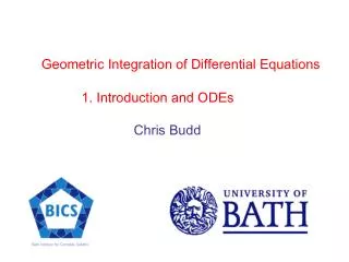
Geometric Integration of Differential Equations 2. Adaptivity, scaling and PDEs Chris Budd
Previous lecture considered constant step sizeSymplectic methods for Hamiltonian ODEs Now we will look at variable step size adaptive methods for ODES We will extend them to scale invariant methods for a wide class of PDES Then look at more general symplectic methods for Hamiltonian PDEs
The need for adaptivity: the Kepler problem Conserved quantities: Hamiltonian Angular Momentum Symmetries: Rotation, Reflexion, Time reversal, Scaling Kepler's Third Law
Kepler orbits FE SE SV
FE Global error SV H error Main error t
Advantages of fixed step Symplectic methods Conservation of L, near conservation of H, shadowing, efficient high order splitting methods. Problemswith fixed step Symplectic methods Larger error at close approaches Kepler’s third law is not respected
Adaptive time steps are highly desirable But … Adaptivity can destroy the shadowing structure [Sanz-Serna] Adaptive methods may not be efficient as a splitting method AIM: To construct efficient, adaptive, symplectic methods EASY
H error t
Symplectic methods and the Sundman transform Hamiltonian system: The Sundman transformis a means of introducing a continuous adaptive time step. IDEA: Introduce a fictive computational time
SMALL if solution requires small time-steps BUT .. rescaling of system is NOT initially Hamiltonian. Use Poincare transformation for Hamiltonian
Good news: Rescaled system is Hamiltonian. Bad news: Hamiltonian is not separable Can’t use efficient splitting methods Method one [Hairer]Use an implicit Symplectic method Method two [Reich, Leimkuhler,Huang]Use an efficient symmetric (non-symplectic ) adaptive Verlet method Method three [B, Blanes]Use a canonical transform to obtain a separable Hamiltonian
Canonical transformation: Introduce new variables (P,Q) for which we have a separable Hamiltonian system. Consider the special scalar case: Theorem: The following transformation is canonical Now find by solving
Choice of the scaling function g(q) Performance of the method is highly dependent on the choice of the scaling function g. There are many ways to do this! One approach is to insist that the performance of the numerical method when using the computational variable should be independent of the scale of the solution
The differential equation system Is invariant under scaling if it is unchanged by the transformation eg. Kepler’s third law relating planetary orbits It generically admitsparticular self-similar solutionssatisfying
Theorem [B, Leimkuhler,Piggott] If the scaling function satisfies the functional equation Then Two different solutions of the original ODE mapped onto each other by the scaling transformation are the same solution of the rescaled system scale invariant A discretisation of the rescaled system admits a discrete self-similar solution which uniformly approximates the true self-similar solution for all time
Example 1: Kepler problem in radial coordinates A planet moving with angular momentum with radial coordinater = qand withdr/dt = psatisfies a Hamiltonian ODE with Hamiltonian If this is invariant under Self-similar collapse solution
If there are periodic solutions with close approaches Hard to integrate with a non-adaptive scheme q t
Consider calculating them using the scaling No scaling Levi-Civita scaling Scale-invariant Constant angle
H Error Method order
1 1.5 1.8 Q P t
Example 2: Motion of a satellite around an oblate planet Integrable if Levi-Civita scaling works best in this case If then scale invariant scaling is best for eccentric orbits
L-C SI eccentricity
Extension of scale invariant methods to PDES These methods extend naturally to PDES with a scaling invariance
Idea: Introduce a computational coordinate And a differential equation linking to X Mesh potential P Monitor function M (large where mesh points need to cluster) Parabolic Monge-Ampere equation PMA
Choose the monitor function M(u) by insisting that the system should be invariant under changes of spatial and temporal scale Example: Parabolic blow-up equation Scaling: Monitor:
Solve PMA in parallel with the PDE 10 10^5 Solution: Y X Mesh:
Solution in the computational domain 10^5 Same approach works well for the Chemotaxis eqns, Nonlinear Schrodinger eqn, Higher order PDEs
More general geometric integration methods for PDES Geometric integration methods for PDES are much less well developed than for ODEs as PDES have a very rich structure and many conservation laws and it is hard to preserve all of this under discretisation Hamiltonian: NLS, KdV, Euler eqns Lagrangian structure: Scaling laws: NLS, parabolic blow-up, Porous medium eqn Conservation laws and integrability: NLS Have to choose what to preserve under discretisation: Variational integrators, scale-invariant, multi-symplectic
Example:Multi-symplectic methods for Hamiltonian PDEs [Bridges, Reich, Moore,Frank, Marsden, Patrick, Schkoller,McLachlan,Ascher] NLWE
Many PDEs have this multi-symplectic form Shallow water, NLS, KdV, Boussinesq They typically have local conservation laws of the form IDEA Discretise these equations using asymplectic method in t and asymplecticmethod in x
Eg. Use the implicit mid-point rule Preissman/Keller Box Scheme
Preissman/Keller Box Scheme • Preserves conservation laws arising from linear symmetries • Preserves energy and momentum for linear PDES • Gives correct dispersion relation for linear equations • Not much known for nonlinear problems Study using backward error analysis: modified equation has a multi-symplectic structure, but don’t get exponentially small estimates.
Conclusion Geometric integration has proved to be a powerful tool for integrating ODEs with many different scales Its potential for PDES is still being developed, but it could have a significant impact on problems such as weather forecasting It is an area where pure mathematicians, applied mathematicians, numerical analysts, physicists etc must all work together