Download
1 / 14
140 likes | 263 Views
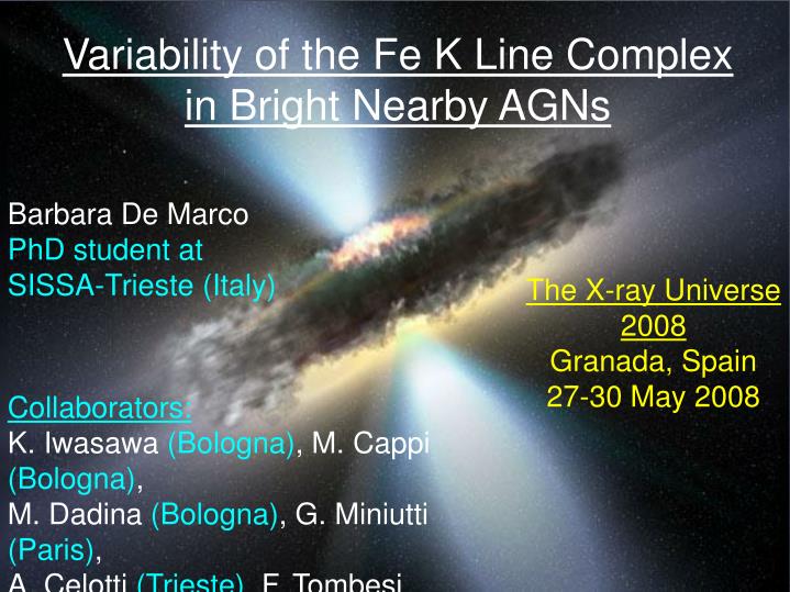
Variability of the Fe K Line Complex in Bright Nearby AGNs. Barbara De Marco PhD student at SISSA-Trieste (Italy). The X-ray Universe 2008 Granada, Spain 27-30 May 2008. Collaborators: K. Iwasawa (Bologna) , M. Cappi (Bologna) , M. Dadina (Bologna) , G. Miniutti (Paris) ,

E N D
Variability of the Fe K Line Complex in Bright Nearby AGNs Barbara De Marco PhD student at SISSA-Trieste (Italy) The X-ray Universe 2008 Granada, Spain 27-30 May 2008 Collaborators: K. Iwasawa (Bologna), M. Cappi (Bologna), M. Dadina (Bologna), G. Miniutti (Paris), A. Celotti (Trieste), F. Tombesi (Bologna)
Why Studying Fe K line variability patterns Relativistic Fe K lines are powerful tools for the study of the inner accretion flow. ✪ Tanaka et al. 1995 They give us the most direct view on the physics in the vicinity of astrophysical Black Holes. ✪ Müller & Camenzind 2004 Variability is useful to understand the dynamics of the flow, the geometry and structure, etc. ✪ Iwasawa et al. 2004
Fe K line variability patterns in literature NCG 3516 [Iwasawa et al. 2004] MKN 766 [Turner et al. 2006 ] NGC 3783 [Tombesi et al. 2007] MKN 841 [Petrucci et al. 2007] ESO 113-G010 [Porquet et al. 2007] ........ !!! No Systematic study on a complete sample does exist !!! XMM-Newton sensitivity and effective area are high enough to provide early indications of orbital-time scale spectral variability [Miller 2007]
The complete sample ✦ Original Sample (proposed in Guainazzi et al. 2006) complete sample of32 sources (selected from the RXTE Slew Survey) for the study of relativistic Fe lines time-averaged properties. -11 2 ✔ Flux limit: F(2-10 keV) ≥1.5x10 erg/cm /s ✔ Cold absorption limit: N < 1.5x10 cm ✔ XMM-Newton observation duration: long enough to collect ≥10 sourcecounts between 2-10 keV 22 2 H 5
Our sample ✔ Observations with public data prior to Jan 2008 ✔ 7 sources excluded because already extensively studied in their Fe K line variability properties* *MCG-6-30-15 [Ponti et al. 2004], NGC 3516 [Iwasawa et al. 2004], NGC 3783 [Tombesi et al. 2007], MKN 766 [Turner et al. 2006], NGC 4051 [Ponti et al. 2006], MKN 509 [Ponti et al. in prep.], ESO 198-G24 [Miniutti et al. in prep.] Final Sample: 11sources (14observations in total) De Marco, Iwasawa, Cappi, Dadina, Miniutti, Celotti & Tombesi 2008 [submitted]
Excess Maps (Iwasawa, Miniutti & Fabian 2004) 3. Excess residuals maps : in the time-energy plane 1. Continuum fit of time resolved spectra (4-9 keV, time resolutions ∼2.5-5 ks): power law + cold absorption excluding the Fe K line complex energy band 2. Excess residuals : data - model 4. Residuals light curves : integration over 3 pre-defined energy bands and plot as a function of time 5. Monte Carlo simulations of 1000 excess maps (assuming constant lines parameters and variable power law normalization): estimate of light curves errors and variability significance Errors: σ =√<σ > Var. significance N : σ ≥σ 2 2 2 sim redshifted Fe Kα r A: 5.4-6.1 keV B: 6.1-6.8 keV C: 6.8-7.2 keV sim sim neutral/mildly ionized Fe Kα highly ionized Fe Kα/Fe Kβ
Results from Excess Maps ✫ 5 sources out of the 11 of our sample show high significance (> 90%) variability ✫ Plus sources already studied: 9 out of 17 have variable Fe lines !! !!! NEW XMM-NEWTON DATA WILL ALLOW TO COMPLETE THE ANALYSIS ON ALL THE 32 SOURCES AND SURVEY A STATISTICALLY COMPLETE SAMPLE FOR TRANSIENT FEATURES!!!
A Case Study for IC 4329a 5.4-6.1 keV feature light curve: variability confidence level 95.6% Excess Map: Search for Intensity Modulation Time-Scale : epoch folding over 26 trial periods (P = 5 - 67.5 ks, ΔP = 2.5 ks) [e.g. Leahy et al. 1983] Test of global significance against white noise: folding of 1000 simulated light curves; distribution of ξ=max{Χ (P)/<Χ (P)>}[Benlloch et al. 2001] P =32.5 ks 0 2 2 P peak significance: 97.8% 0
A Case Study for IC 4329a Detrended Continuum Light Curve (subtraction of low frequency variability components) τ =15 ks Discrete Cross Correlation Function [Edelson & Krolik 1988] Significant at ∼97% confidence level against white noise 2.3σ (causally unrelated time series)
A Case Study for IC 4329a ✦ The Fe line power spectrum (PSD) is unknown!!! ✦ASSUMPTION: the Fe K line has the same red noise PSD as the continuum ✦ Typical power law index values: β∼1.0-2.0 (Uttley & McHardy 2004) 0.3-10 keV continuum light curve PSD (with fractional rms squared normalization): integration over a small interval of frequencies around 1/P gives a 3% fractional rms << feature light curve relative error (∼63%) 0 ✧ CONCLUSION: negligible contribution from the red noise component to the observed variability !!!
A Case Study for IC 4329a ✦ 2nd ASSUMPTION: variability amplitude of the red noise component is of the same order of the feature one (rms∼60%) - simulation of 1000 light curves with RED + WHITE noise PSD (Timmer & König 1995) - adopted PSD template: N (ν +σ ) , with β=1.3 - Global significance test for intensity modulation: - Time lag significance test (simulated and continuum light curves CCF): -β 2 ✫ P Peak significance: 95.7% 0 ✦ β=1.0-2.0 --->Peak significance:∼95%-96%(almost independent on the choice of β) ✫ Time lag significance: 96.6%
A model for IC 4329a ✦ Intensity modulation time-scale (P ∼32.5 ks): - estimate of the Keplerian orbital radius of the emitting material T = 310 [a + (r/r ) ] M sec ✫ r∼22 r (for M =9.9x10^6 M , Peterson et al. 2004) 0 3/2 g 7 g ⦿ BH ✦ Time lag (τ∼15 ks): - estimate of the distance between the production sites of continuum and line emission: τ = 2d (cos i)/c sec ✫ d∼150-300 r (for a disk i=0 -60 and M =9.9x10^6 M ) ° ° g ⦿ BH
A model for IC 4329a ✦ Intensity modulation --> consistent with the “orbiting spot” scenario (e.g. Dovčiak et al. 2004, Goosmann et al. 2006) BUT ✦ Flare models assume a X-ray source located at few r from the disk (Nayakshin & Kazanas 2001) --> at odd with the distance derived from CCF time lag ✦ In orbiting spot scenarios energy modulations are also expected --> not detected (as for NGC 3783, Tombesi et al. 2007) HENCE ✫ IC 4329a variability pattern not consistent with standard interpretations ✫ Support to models which locate the X-ray source at more elevated heights (like lamp-post models, e.g. Reynolds et al. 1999) g
Thank you! Acknowledgements: BDM is grateful to ESA and ESA Education for grant support