Download
1 / 71
710 likes | 887 Views
X. v. v. X-p. X-pp. v. v. Y. v. v. Y-p. Y-pp. v. v. Etc. 6.8 Double phosphorylation in protein kinase cascades: Protein kinases X,Y and Z are usually phosphorylated on two sites, and often require both phosphorylations for full activity. 6.9 Multi-layer perceptrons

E N D
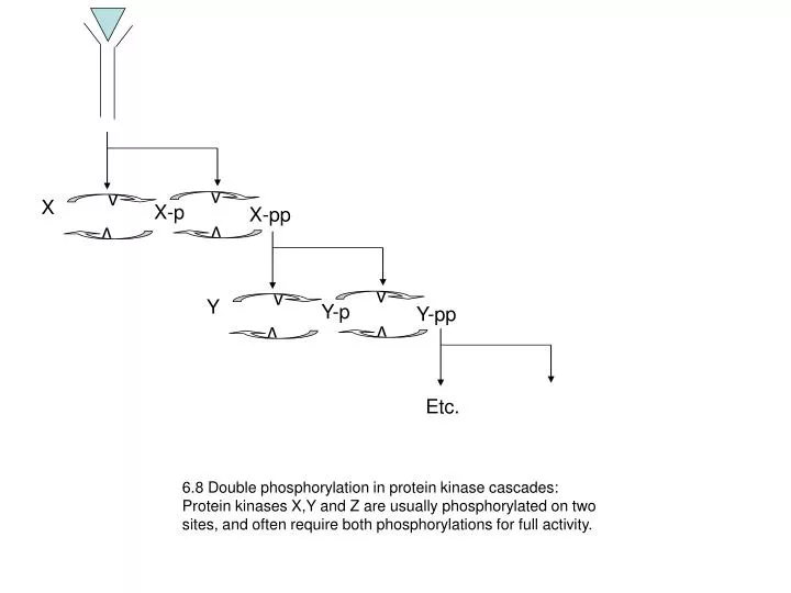
X v v X-p X-pp v v Y v v Y-p Y-pp v v Etc. 6.8 Double phosphorylation in protein kinase cascades: Protein kinases X,Y and Z are usually phosphorylated on two sites, and often require both phosphorylations for full activity.
6.9 Multi-layer perceptrons In protein kinase cascades. Several different receptors in the same cell can activate specific top-layer kinases in response to their ligands. Each layer in the cascade often has multiple kinases, each of which can phosphorylate many of the kinases in the next layer. v v X1 X1-p X2 X2-p v v Phosphatase v Y1 Y1-p v Y2 Y2-p v v v Z1 Z1-p v Z2-p Z2 v v
Fig 6.10: Fraction of active Y as a function of the weighted sum of the input kinase activities, w1 X1 + w2 X2, in the model with first order kinetics. Shown Is the activation curve for single and double phosphorylation of Y. The weights W1 and w2 are the ratio of the input kinase velocity and the phosphatase rate. Fraction of Active Y Single phos. Yp X2 X1 W1 W2 Y Double phos. Ypp Summed input kinase activity w1X1+w2X2
a) b) X2 X1 X2 X1 W1=2 W2=2 W1=0.7 W2=0.7 Y Y X2 X2 X1 X1 Fig 6. 11 Single-layer perceptrons and their input functions. Node Y sums the two inputs X1 and X2 according to the weights w1 and w2. Y is activated in the colored region of the X1-X2 plane. In this region w1X1+w2X2>1. In protein kinase cascades, Y is phosphorylated and hence active in the shaded region. In this figure, as well as Fig 6.12-6.13, the range of activities of X1 and X2 is assumed to be between zero and one. Activity of one means that all input kinase molecules is active. This defines the square region in X1-X2 plane portrayed in the figures.
X2 X1 X2 X1 1.5 b) 1.5 a) 0.7 0.7 0.7 1.5 0.7 1.5 Y1 Y2 Y1 Y2 0.6 0.6 2 2 Z Z x2 x2 Y1 Y2 Y1 Y2 x1 x1 x2 x2 Z Z x1 x1 Fig 6. 12 Two-layer perceptrons and their input functions. (a) Y1 and Y2 are active (phosphorylated) in the shaded regions, bounded by straight lines. The weights of Z are such that either Y1 or Y2 Y is activated (phosphorylated above threshold) in the colored regions of the X1-X2 plane. In this region w1X1+w2X2>1. (b) Here the weights for Z activation by Y1 and Y2 are such that both Y1 and Y2 need to be active. Hence the activation region of Z is the intersection of the activation regions of Y1 and Y2.
X2 X1 X2 X1 0.7 1.5 0.7 1.7 0.7 1.7 0.7 1.5 Y1 Y2 Y1 Y2 2 -3 -3 2 Z Z Y2 Y1 Y1 Y2 Z Z Fig 6. 13 Two-layer perceptrons and their input functions. Y1 and Y2 are active in the shaded regions, bounded by straight lines. (a) Y1 activates Z whereas Y2 inhibits it (eg a phosphatase). Thus, Z is activated in a wedge-like region in which Y1 is active but Y2 is not. (b) and additional example that yields an output Z that is activated when both inputs are intermediate, when either X1 or X2 are highly active, but not both (similar to an exclusive-OR gate).
X Bacteria Fruit-Flies Yeast sH Ime1 smo dnaK dnaJ Ime2 Ptc Mammals HSF1 NFkB HIF p53 hsp70 hsp90 IkB iNOS Mdm2 (a) 6.14 Composite network motifs made of transcription interactions (full arrows) and protein-protein interactions. (dashed arrows). (a) Transcription factor X regulates two genes Y and Z, whose protein products interact. (b) A negative feedback loop with one transcription arm and one protein arm is a common network motif across organisms Y Z (b) x y
6.15 Negative feedback in engineering uses fast control on slow devices. A heater, which can heat a room in 15 minutes, is controlled by a thermostat that compares the desired temperature to the actual temperature. If the temperature is too high, the power to the heater is reduced, and power is increased if temperature is too low. The thermostat works on a much faster timescale than the heater. Engineers tune the feedback parameters to obtain rapid and stable temperature control (and avoid oscillations). Heater Power supply Temperature slow Thermostat fast
6.16 Negative feedback can show over-damped, monotonic dynamics (blue), damped oscillations with peaks of decreasing amplitude (red) or undamped oscillations (green dashed line). Generally, the stronger the interactions between the two nodes in relation to the damping forces on each node (such as degradation rates), the higher the tendency for oscillations.
a) Oscillator motif Repressilator b) Z X X Y Y Fig 6.17 A network motif found in many biological oscillatory systems, composed of a composite negative feedback loop and a positive auto-activation loop. In this motif, X activates Y on a slow timescale, and also activates itself. Y inhibits X on a rapid timescale. (b) A repressilator made of three cyclically linked inhibitors shows noisy oscillations In the presence of noise in the production ratesfor a wide range of biochemical parameters.
Fig 6.18 Network motifs found in different networks (Milo et al Science 2002) Developmental Transcription Networks X X X Y Z Z X Y Y Y Z Z
Fig 6.19 Significance profiles of three-node subgraphs found in different networks. The significance profile allows comparison of networks of very different sizes ranging form tens of nodes (social networks where children in a school class select friends) to millions of nodes (world-wide-web networks). The y-axis is the normalized Z-score (Nreal-Nrand) / std(Nrand) for each of the thirteen three-node subgraphs. Language networks have words as nodes and edges between words that tend to follow each other in texts. The neural network is from C. elegans (chapter 6), counting synaptic connections with more than 5 synapses. For more details, see Milo et al Science 2004.
6.20 Map of synaptic connections between C. elegans neurons. Shown are connections between neurons in the worm head.Source: R. Durbin PhD Thesis, www.wormbase.org
ASH Nose touch Noxious chemicals, nose touch Sensory neurons FLP AVD Interneurons AVA Backward movement Thomas & Lockery 1999 6.21 Feed-forward loops in C. elegans avoidance reflex circuit. Triangles represent sensory neurons, hexagons Represent inter-neurons. Lines with triangles represent synaptic connections between neurons.
(a) Fig 6.22: Dynamics in a model of a C. elegans multi-input FFL following pulses of input stimuli. a) A double input FFL, input functions and thresholds are shown. b) Dynamics of the two-input FFL, with well-separated input pulses For X1 and X2, followed by a persistent X1 stimulus. C) Dynamics With short X1 stimulus followed rapidly by a short X2 stimulus. The dashed horizontal line corresponds to the activation thresholds for Y. a=1 was used. Dynamics (b) Source: Kashtan et al, PRE 2004 70: 031909 (c)
b c a d f h g e k n m j l i Fig 6.23 Five and six node network motifs in the neuronal synaptic network Of C. elegans. Note the multi-layer perceptron patterns e,f,g,h,k,l,m and n, many of which have mutual connections within the same layer. The parameter C is the concentrationof the subgraph relative to all subgraphs of the same size in the network (multiplied by 10^-3), Z is the number of standard deviations it exceeds randomized networks With the same degree sequence (Z-score). These motifs were detected by an efficient sampling algorithm suitable for large subgraphs and large networks. Source: N. Kashtan, S. Itzkovitz, R. Milo, U. Alon, Efficient sampling algorithm for estimating subgraph concentrations and detecting network motifs. Bioinformatics. 2004 Jul 22;20(11):1746-58.
The bacteria flagella motor [source: Berg HC, Ann. Rev. Biochem 2003] Fig 7.3
Run Tumble Motors turn CCW Motor turns CW When tethered to a surface the entire cell rotates, and Individual motors show two-state behavior CCW CW 10 sec time Fig 7.4 Bacterial runs and tumbles are related to the rotation direction of the flagella motors. When all motors spin counter-clockwise (CCW), the flagella turn in a bundle and cell is propelled forward. When one or more motors turn clockwise (CW), the cell tumbles and randomizes its orientation. . The switching dynamics of a single motor from CCW to CW and back can be seen by tethering a cell to a surface by means of its flagellum, so that the motor spins the entire cell body (at frequencies of a few hertz due to the large viscous drag of the body).
Tumbling frequency Attractant added 1/sec exact adaptation Time [min] Fig 7.5 : Average tumbling-frequency of a population of cells exposed at time t= 5 to a step addition of saturating attractant (such as L-aspartate). After t=5, attractant is uniformly present at constant concentration. Exact adaptation means that the steady-state tumbling-frequency does not depend on the level of attractant.
Fig 7.6 The chemotaxis signal transduction network [source: Alon et al Nature 1999]
m m Fig 7.7 Fine-tuned mechanism for exact adaptation. Receptors are methylaed by CheR and de-methylated by CheB. Methylated receptors (marked with an m) catalyze the phsophorylation of CheY, leading to tumbles. When attractant binds, the activity of each methylated receptors is reduced. In addition, the velocity of the CheB enzyme is reduced due to its reduced phosphorylation. Thus, the concentration of methylated receptors increases, until the tumbling frequency returns to the pre-stimulus state. Exact adaptation depends on tuning between the reduction in CheB velocity and the reduction in activity per methylated receptor upon attractant binding, so that the Activity per methylated receptor times the number of methylated receptors Returns to the pre-stimulus level.
A a) A b) Adaptation is not exact time time Figure 7.8: Activity dynamics in the fine-tuned model in response to a step addition of saturating attractant At time t=2 (dimensionless units throughout). A) Fine-tuned model shows exact adaptation with a tuned parameter set B) Dynamics when CheR level is lowered by 20% with respect to the tuned parameter set of A.
m m Fig 7,9 Robust mechanism for exact adaptation. Un-methylated receptors are methylated by CheR at a constant rate. Methylated receptors (marked with m) transit rapidly between active and inactive states (the former marked with a star). Attractant binding increases the rate to become inactive, whereas repellents increase the rate to become active. De-methylation is due to CheB, which acts only on the active methylated receptors. The active receptors catalyze the phosphorylation of CheY, leading to tumbles. Exact adaptation occurs when the concentration of active receptors Adjusts itself so that the de-methylation rate is equal to the constant methylation rate.
a) b) A A time time Fig 7.10: Activity dynamics of the robust model in response to addition of saturating attractant at time t=2. a) model parameters K=10, VR R =1, VB B=2. b) same parameters with R reduced by 20%. Exact adaptation is preserved. Note that the steady-state tumbling frequency is fine-tuned, and Depends on the model parameters.
adaptation time steady-state tumbling freq. Fig 7.11. Experimental test of robustness in bacterial chemotaxis. The protein CheR was expressed at different levels by means of controlled expression with an inducible promoter, and the average tumbling frequency of a cell population was measured using video microscopy. Fold-expression is the ratio of CheR protein level to that in the wild-type bacterium. Adaptation time and steady-state tumbling frequency varied with CheR, whereas adaptation remained exact. Adaptation precision is the ratio of tumbling frequency before and after saturating attractant (1mM aspartate). Wild-type tumbling frequency in this experiment is about 0.4/sec (black dot in b). Source: Alon, Barkai, Surette, Leibler, Nature 1999.
Morphogen Concentration M 1 0.8 0.6 Threshold 1 Threshold 1 0.4 Threshold 2 0.2 Region A Region A Region B Region B Region C Region C 0 0 0.5 1 1.5 2 2.5 3 Position, X Fig 8.1 Morphogen gradient and the French flag model. Morphogen M is Produced at x=0, and diffuses into a field of cells. The morphogen is degraded As it diffuses, resulting in a steady state concentration profile that decays With distance from the source at x=0. Cells in the field assume fate A if M concentration is greater than threshold 1, fate B if M is between threshold 1 and 2, and fate C if M is lower than threshold 2.
Mo Morphogen Concentration M(x) M’o Threshold T δ Xo X’o Position x Fig 8.2: Changes in steady-state morphogen profile and the resulting pattern boundary upon a two-fold reduction in morphogen concentration at x=0, Mo. The pattern boundary, defined by the position where M equals the threshold T, shifts to the left by δ .
Mo M(x) Morphogen concentration M’o M(x)=Mo Shift, δ Position x Fig 8.3, A change in morphogen concentration at th source from Mo to Mo’ leads to a spatially uniform shift in the morphogen profile. All arrows are of equal length. The size of the shift is equal to the position at which M(x)=Mo’.
Fig 8.4 Comparison of properties of exponential and power-law morphogen profiles. A diffusible morphogen that is subject to linear degradation reaches an exponential profile at steady state (solid line). A perturbed profile (dashed line) was obtained by reducing the morphogen at the boundary, Mo, by a factor e. The resulting shift in cell fate boundary (δ ) is comparable to the distance between two boundaries in the unperturbed profile (Δx). Note the logarithmic scale. (b) When the morphogen undergoes nonlinear self-enhanced degradation, a power-law morphogen profile is established at steady-state. In this case, δ is significantly smaller than Δx. The symbols are the same as in (a), and quadratic degradation was used (Eq 8.7). M δ δ M Source: Eldar et al Dev Cell. 2003 Oct;5(4):635-46.
b) a) M degradation M degradation R R Fig 8.5 Two network motifs that provide self enhanced degradation of morphogen M. (a) Mbinds receptor R and activates signaling pathways that increase R expression. M bound to R is taken up by the cells (endocytosis) and M is degraded. (b) M binds R and activates signaling pathways that repress R expression binds and sequesters an extra-cellular protein that degrades M (a protease), thus R effectively inhibits M degradation.
Fig 8.6: Cross section of the early drosophila embryo, about 2h from start of development. Cells are arranged on the periphery of a cylinder. Three cell types are found ( three distinct domains of gene expression) This sets the stage for the patterning considered in this section, in which the dorsal region (DR), which comprises about 50 cells, is to be Sub-patterned. Shown are the regions of expression of the genes of the patterning network: M is the morphogen (Scw, an activating BMP class ligands, also Dpp, expressed in DR); I is an inhibitor of M (Sog); P is a protease (Tld) that cleaves I. Note that M is expressed by all cells, P is expressed only in DR , and expression of I is restricted to the neuroectoderm (NE). (b) Robustness of signaling pathway activity profile in the DR. Pathway activity corresponds to the level of free of M. Robustness Was tested with respect to changes in the gene dosage of M,I and P. Shown are measurement of signaling pathway activity for wild-type cells and mutants with half gene dosage for M (scw+/-) ,I (sog+/-)and P(tld+/-), as well as over-expressed P (tld OE). P P--| I --| M M I I Source: Eldar A, Dorfman R, Weiss D, Ashe H, Shilo BZ, Barkai N. Nature. 2002 Sep 19;419(6904):304-8. DR
free Morphogen (unbound to inhibitor) inhibitor Position along dorsal region Fig 8.7: Simple model for patterning of the dorsal region. Inhibitor is produced at the boundaries of the region, at x=-1 and x=1. Inhibitor is degraded, and thus its concentration decays into the dorsal region. Free morphogen, unbound to inhibitor, is thus highest at the center of the region, at x=0.
Fig 8.8: Patterning in non-robust and robust mechanisms. . a, Profile of free M in a typical non-robust network. The profile of free M (bold curve) is shown for the non-perturbed network and for three perturbed networks representing half-production rates of M, I and P (dotted, dot-dash and dashed lines). The total concentration of M (free and bound to I, M+[MI]) is indicated by the grey line (arrow). The broken grey line (T) indicates the threshold where robustness was measured. b, Profile of free M in a typical robust system (note logarithmic scale on the y axis). Source: Eldar A, Dorfman R, Weiss D, Ashe H, Shilo BZ, Barkai N. Nature. 2002 Sep 19;419(6904):304-8.
Correct tRNA+amino-acid Incorrect tRNA +amino acid Elongating protein chain (linked amino-acids) Kc Kd mRNA Ribosome Fig 9.1: Translation of a protein at the ribosome. The mRNA is read by tRNAs that specifically recognize triplets of letters on the mRNA called codons. When a tRNA binds the codon, the amino acid that it carries links to the elongating protein chain. The tRNA is ejected and the next codon is read. Each tRNA competes for binding with the other tRNA types in the cell. The correct tRNA binds with dissociation Constant Kc, whereas the closest incorrect tRNA binds with Kd>Kc.
Fig 9.1b: The ‘universal’ genetic code. Shading indicates polar requirement (PR)1: lighter shades (black text), PR , 6 (hydrophobic); medium shades (yellow text), PR 5 6–8 (medium); darker shades (white text) PR . 8 (hydrophilic). From Knight Freeland and Landweber, TIBS 24, 1999.
Fig 9.2 Recognition of foreign peptides by T-cells. Target cells present Fragments of their proteins bound to MHC proteins on the cell surface. Each T-cell can recognize specific foreign peptides by means of its T-cell receptor. Recognition can result in killing of the target cell by the T-cell.
P P P P P P P P Signaling Fig 9.2 Kinetic proofreading model in T-cell receptors. Ligand binding Initiates modifications to the receptors. When sufficient modifications have occurred, signaling pathways are triggered in the cell. At any stage, ligand can dissociate from the receptor, resulting in immediate loss of all of the modifications. The series of modifications Creates a delay between ligand binding and signaling. Only ligands that remain bound throughout this delay can trigger signaling.
d∙ZWT 10.1 Benefit of Lac proteins of E. coli as a function of lactose. Cells were grown with saturating IPTG and varying levels of lactose. Growth rate difference is shown relative to the growth rate of cells grown with no IPTG or lactose. Benefit= δ *L*L/(K+L) δ ZwT~0.17is the benefit of lac induction at saturating lactose levels. Red line: theoretical growth rate, Eq 10.2.4. Source: Dekel & Alon Nature 2005
0.08 0.06 (relative growth rate reduction) 0.04 0.02 h cost, 0 0 0.5 1 1.5 Relative lac expression (Z/Z ) W T 10.2 Cost of lac proteins in wild-type E. coli. The cost is defined as relative reduction in growth of E. coli wild-type cells grown in defined glycerol medium with varying amount of IPTG relative to cells grown with no IPTG. The x-axis is LacZ protein level relative to LacZ protein level at saturating IPTG (ZWT). Also shown are the cost of strains evolved at 0.2mM lactose for 530 generations (data point at 0.4∙ZWT, open triangle) and 5mM lactose for 400 generations (data points at 1.12·ZWT open triangle). Red line: theoretical cost Function Eq 10.2.3. COST=h*Z/(1-Z/M)
10.3 Predicted relative growth rate of cells (the 'fitness function') as a function of Lac proteinexpression, in different concentrations of lactose, based on the experimentally measured cost and benefit functions. The x-axis is the ratio of protein level to the fully induced wild-type protein level, Z/ZWT. Shown are relative growth differences with respect to the un-induced wild-type strain, for environments with lactose levels L=0.1mM (blue line), L=0.6 mM (green line) and L=5mM (red Line), according to Eq (5). The dot on each line is the predicted optimal expression level which provides maximal growth, Eq 6. Cells grown in lactose levels above 0.6mM are predicted to evolve to increased Lac protein expression (top arrow ), whereas cells grown at lactose levels lower than 0.6mM are predicted to evolve to decreased expression (lower arrow ) .
1.2 1 0.8 Normalized LacZ protein level 0.6 0.4 0.2 0 0 1 2 3 4 5 6 L(mM) 10.4 Adapted LacZ activity of cells in serial-dilution experiments as a function of the lactose concentration in the environment L, relative to wild-type cells. Data is for 530 generations, except for the data point at 5mM lactose which is at generation 400. Red line: Theoretical prediction for optimal expression level, (Eq. 10.2.6).
1.2 5mM Lactose 2mM Lactose 1 0.5mM Lactose 0.8 LacZ Protein Level 0.6 0.1mM Lactose No Lactose 0.4 0.2 0 100 200 300 400 500 Generations :10.5 Experimental evolutionary adaptation ofE. coli cells to different concentrations of lactose. LacZ activity relative to wild-type cells of cells grown for 530 generations in serial dilution experiments with different lactose levels is shown as a function of generation number. Cells were grown in 0,0.1mM,0.5mM,2mM and 5mM lactose in a glycerol minimal medium supplemented with 0.15mM IPTG. Lines are population genetics simulations of the serial dilution conditions. The only fitting parameter in these simulations is the probability per cell division for a mutation that yields the adapted lacZ level.
Variable environment • Suppose Z is produced with benefit only in the environment condition Cz with prob. p • Three strategy:1. Unregulated f1=p*b-c2. Regulated f2=p*b-c*p-r3. Lack of gene Z f3=0 no benefit b no cost c
Variable environment • Regulation wins: f2> f1 and f2>f3p<1-r/c and p > r/(b-c) • Non regulation wins:p > c/b and p > 1- r/c
Variable environment • If p=1 always Cz Z should be always expressed (f1 best) • If p=0 Cz never happens and Z should not be expressed (f3 best) • If the environment is sufficiently variables f2 is the best
r/c 1 System always OFF System always ON Relative cost of regulatory system Regulation 0 0 p 1 Demand for X in the environment Fig 10.6: Selection phase diagram, showing regions where gene regulation, genes always ON or genes always OFF are optimal. The x-axis is the fraction of time p that the environment shows conditions in which the protein X is needed, and brings benefit (p is called the demand for X). The ratio of protein cost to regulation system cost is r/c.