Download
1 / 43
430 likes | 449 Views
Explore the role of graph algorithms in network problems, from routing to shortest path computation. Learn about Distributed Bellman-Ford, OSPF, AS, and more. Discover efficient solutions for network optimization.

E N D
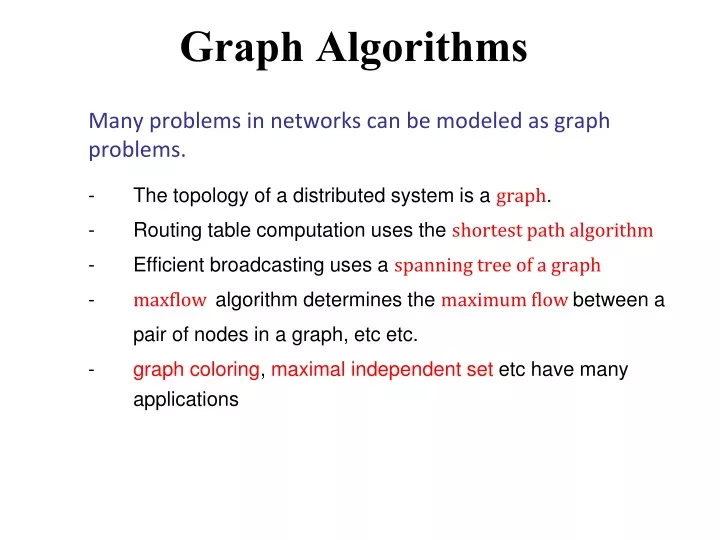
Graph Algorithms Many problems in networks can be modeled as graph problems. - The topology of a distributed system is a graph. - Routing table computation uses the shortest path algorithm - Efficient broadcasting uses a spanning tree of a graph - maxflow algorithm determines the maximum flow between a pair of nodes in a graph, etc etc. - graph coloring, maximal independent set etc have many applications
Routing • Shortest path routing • Distance vector routing • Link state routing • Routing in sensor networks • Routing in peer-to-peer networks
Internet routing Autonomous System Autonomous System AS1 AS0 Each belongs to a single administrative domain Autonomous System Autonomous System AS2 AS3 Intra-AS vs. Inter-AS routing Open Shortest Path First (OSPF) is an adaptive routing protocol for Internet Protocol (IP) network
Routing: Shortest Path Classical algorithms like Bellman-Ford, Dijkstra’s shortest-path algorithm etc are found in most algorithm books. In a distributed graph algorithm only one node and its neighbors are visible to a process In an (ordinary) graph algorithm the entire graph is visible to the process
Most distributed algorithms for shortest path are adaptations of Bellman-Ford algorithm. It computes single-source shortest paths in a weighted graphs. Designed for directed graphs. Computes shortest path if there are no cycle of negative weight. Let D(j) = shortest distance of node j from initiator 0. D(0) = 0. Initially, ∀i ≠ 0, D(i) =∞. Let w(i, j) = weight of the edge from node i to node j Routing: Shortest Path Sender’s id w(0,m),0 initiator 0 m (w(0,j), 0 j (w(0,j)+w(j,k)), j (w(0,j)+w(j,p)), j Parent relation k p The edge weights can represent latency or distance or some other appropriate parameter.
Distributed Bellman Ford: Consider a static topology {Process 0 sends w(0,i),0 to each neighbor i} {program for process i} do message = (S,k) ∧ S < D(i) if parent ≠ k parent := k fi; D(i) := S; send (D(i)+w(i,j),i) to each neighbor j ≠ parent; [] message (S,k) ∧ (S ≥ D(i)) skip od Shortest path Current distance Computes the shortest distance from all nodes to the initiator node The parent links help the packets navigate to the initiator
Shortest path Synchronous or asynchronous? The time and message complexities depend on the model. The goal is to lower the complexity [Synchronous version] In each round every process i sends out D(i) + w(i,j),j to each neighbor j Observation: for a node i, once D(parent(i)) becomes stable, it takes one more round for D(i,0) to be stable Time complexity = O(diameter) rounds Message complexity = O(|V|)(|E|)
Complexity of Bellman-Ford Theorem.The message complexity of asynchronous Bellman-Ford algorithm is exponential. Proof outline. Consider a topology with an odd number nodes 0 through n-1 (the unmarked edges have weight 0) n-4 n-2 1 3 5 20 2k 2k-1 22 21 n-5 n-3 n-1 0 4 2 An adversary can regulate the speed of the messages D(n-1) reduces from (2k+1- 1) to 0 in steps of 1. Since k = (n-3)/2, it will need 2(n-1)/2-1 messages to reach the goal. So, the message complexity is exponential.
Chandy & Misra’s algorithm : basic idea (includes termination detection) Process 0 sends w(0,i),0 to each neighbor i {for process i > 0} do message = (S ,k) ∧ S < D if parent ≠ k send ack to parent fi; parent := k; D := S; send (D + w(i,j), i) to each neighbor j ≠ parent; deficit := deficit + |N(i)| -1 [] message (S,k) ∧ S ≥ D send ack to sender []ack deficit := deficit – 1 [] deficit = 0 ∧ parent ≠ i send ack to parent od Shortest path 0 2 1 7 1 2 3 2 4 7 4 2 6 6 5 3 Combines shortest path computation with termination detection. Termination is detected when the initiator receives ack from each neighbor
Shortest path An important issue is: how well do such algorithms perform when the topology changes? No real network is static! Let us examine distance vector routing that is adaptation of the shortest path algorithm
Distance Vector D for each node i contains N elements D[i,0], D[i,1], … D[i, N-1]. Here, D[i,j] denotes the distance from node i to node j. - Initially ∀i, D[i,j] =0 when j=i D(i,j) = 1 when j ∈N(i). and D[i,j] = ∞ when j ∉ N(i) ∪{i} - Each node j periodically sends its distance vector to its immediate neighbors. - Every neighbor i of j, after receiving the broadcasts from its neighbors, updates its distance vector as follows:∀k ≠ i: D[i,k] = minj(w[i,j] + D[j,k] ) Used in RIP, IGRP etc Distance Vector Routing
Assume that each edge has weight = 1. Currently, Node1: d(1,0) = 1, d(1, 2) = 1, d(1,2) = 2 Node 2: d(2,0) = 1, d(2,1) =1, d(2,3) = 1 Node 3: d(3,0) = 2, d(3,1) = 2, d(3,2) = 1 What if the topology changes?
Node1 thinks d(1,3) = 2 (old value) Node 2 thinks d(2,3) = d(1,3) +1 = 3 Node 1 thinks d(1,3) = d(2,3) +1 = 4 and so on. So it will take forever for the distances to stabilize. A partial remedy is the split horizon method that prevents node 1 from sending the advertisement about d(1,3) to 2 since its first hop (to 3) is node 2 Counting to infinity Observe what can happen when the link (2,3) fails. D[j,k]=3 means j thinks k is 3 hops away ∀k≠ i: D[i,k] = minj(w[i,j] + D[j,k] ) Suitable for smaller networks. Larger volume of data is disseminated, but to its immediate neighbors only. Poor convergence property.
Each node i periodically broadcasts the weights of all edges (i,j) incident on it (this is the link state) to all its neighbors. Each link state packet (LSP) has a sequence number seq. The mechanism for dissemination is flooding. This helps each node eventually compute the topology of the network, and independently determine the shortest path to any destination node using some standard graph algorithm like Dijkstra’s. Link State Routing Smaller volume data disseminated over the entire network Used in OSPF of IP
Link State Routing: the challenges (Termination of the reliable flooding) How to guarantee that LSPs don’t circulate forever? A node forwards a given LSP at most once. It remembers the last LSP that it forwarded for each node. (Dealing with node crash) When a node crashes, all packets stored in it may be lost. After it is repaired, new packets are sent with seq = 0. So these new packets may be discarded in favor of the old packets! Problem resolved using TTL See: http://www.ciscopress.com/articles/article.asp?p=24090&seqNum=4
Conventional routing tables have a space complexity O(n). Can we route using a “smaller” routing table? This is relevant since the network sizes are constantly growing. One solution interval routing. Interval Routing (Santoro and Khatib)
Determine the interval to which the destination belongs. For a set of N nodes 0 . . N-1, the interval [p,q)between p and q (p, q < N) is defined as follows: if p < q then [p,q) = p, p+1, p+2, .... q-2, q-1 if p ≥ q then [p,q) = p, p+1, p+2, ..., N-1, N, 0, 1, ..., q-2, q-1 Interval Routing: Main idea [5,1) [3,5) [1,3)
Example of Interval Routing N=11 Labeling is the crucial part
Labeling algorithm Label the root as 0. Do a pre-order traversal of the tree. Label successive nodes as 1, 2, 3 For each node, label the port towards a child by the node number of the child. Then label the port towards the parent by L(i) + T(i) + 1 mod N, where - L(i) is the label of the node i, - T(i) = # of nodes in the subtree under node i (excluding i), Question 1. Why does it work? Question 2. Does it work for non-tree topologies too? YES, but the construction is a bit more complex.
Anotherexample Interval routing on a ring. The routes are not optimal. To make it optimal, label the ports of node i with i+1 mod 8 and i+4 mod 8.
Example of optimal routing Optimal interval routing scheme on a ring of six nodes
So, what is the problem? Works for static topologies. Difficult to adapt to changes in topologies. Some recent work on compact routing addresses dynamic topologies (Amos Korman, ICDCN 2009)
Prefix routing Easily adapts to changes in topology, and uses small routing tables, so it is scalable. Attractive for large networks, like P2P networks. Label the root by λ, the empty string Label each child of node with label L by L.x (x is a unique for each child. Label the port to connecting to a child by the label of the child. Label the port to the parent by λ When new nodes are added or existing nodes are deleted, changes are only local. a.a.a a.a.b
Prefix routing {A packet arrives at the current node} {Let X = destination, and Y = current node} if X=Y local delivery [] X ≠ Y Find a port p labeled with the longest prefix of X Forward the message to p fi λ = empty symbol
Prefix routing for non-tree topology Does it work on non-tree topologies too? Yes. Start with a spanning tree of the graph. If (u,v) is a non-tree edge, then the edge label from u to v = v, and the edge label from u to its parent = λ unless (u, root) is a non-tree edge. In that case, label the edge from u towards the root by λ, andthe edge label from u to its parent or neighbor v by v a b λ λ a b a.b a.a a.b.a a.b λ b a.a λ b a.b.a a.a.a a.a.a a.b.a λ λ a.b a.b a.a.a
Routing in P2P networks: Example of Chord • Small routing tables: log n • Small routing delay: log n hops • Load balancing via Consistent Hashing • Fast join/leave protocol (polylog time)
Consistent Hashing Assigns an m-bit key to both nodes and objects from. Order these nodes around an identifier circle (what does a circle mean here?) according to the order of their keys (0 .. 2m-1). This ring is known as the Chord Ring. Object with key k is assigned to the first node whose key is ≥ k (called the successor node of key k)
Consistent Hashing (0) D120 N105 D20 N=128 Circular 7-bit ID space N32 N90 D80 Example: Node 90 is the “successor” of document 80.
Consistent Hashing [Karger 97] Property 1 If there are N nodes and K keys, then with high probability, each node is responsible for (1+∊ )K/N keys. Property 2 When a node joins or leaves the network, the responsibility of at most O(K/N) keys changes hand (only to or from the node that is joining or leaving. When K is large, the impact is quite small.
Consistent hashing Key 5 K5 Node 105 N105 K20 Circular 7-bit ID space N32 N90 K80 A keyk is stored at its successor (node with key ≥ k)
The log N Fingers N120 112 ½ ¼ 1/8 1/16 1/32 1/64 1/128 N80 Finger i points to successor of n+2i
Chord Finger Table N32’s Finger Table (0) N113 33..33 N40 34..35 N40 36..39 N40 40..47 N40 48..63 N52 64..95 N70 96..31 N102 N102 N=128 N32 N85 N40 N80 N79 N52 Finger table actually contains ID and IP address N70 N60 Node n’s i-th entry: first node with id ≥ n + 2i-1
Routing in Peer-to-peer networks destination 130102 source 203310 13010-1 1301-10 Pastry P2P network 130-112 13-0200 1-02113
Skip lists and Skip graphs • Start with a sorted list of nodes. • Each node has a random sequence number of sufficiently large length, called its membership vector • There is a route of length O(log N) that can be discovered using a greedy approach.
-∞ +∞ Skip List (Think of train stations) L3 L2 -∞ 31 +∞ L1 -∞ 23 31 34 64 +∞ L0 -∞ 12 23 26 31 34 44 56 64 78 +∞ Example of routing to (or searching for) node 78. At L2, you can only reach up to 31.. At L1 go up to 64, As +∞ is bigger than 78, we drop down At L0, reach 78, so the search / routing is over.
Properties of skip graphs • Skip graph is a generalization of skip list. • Efficient Searching. • Efficient node insertions & deletions. • Locality and range queries.
Routing in Skip Graphs W G Level 2 A J M R 101 100 000 001 011 110 100 G R W Level 1 A J M 110 101 001 001 011 Membership vectors A J M R W Level 0 G 001 001 100 011 110 101 Random sequence numbers Link at level i to nodes with matching prefix of length i. Think of a tree of skip lists that share lower layers.
Properties of skip graphs • Efficient routing in O(log N) hops w.h.p. • Efficient node insertions & deletions. • Independence from system size. • Locality and range queries.
Chang’s algorithm {The root is known} {Uses probes and echoes, and mimics the approach in Dijkstra-Scholten’s termination detection algorithm} {initially ∀i, parent (i) = i} {program of the initiator} Send probe to each neighbor; donumber of echoes ≠ number of probes echo received echo := echo +1 probe received send echo to the sender od {program for node j, after receiving a probe } first probe --> parent: = sender; forward probe to non-parent neighbors; donumber of echoes ≠ number of probes echo received echo := echo +1 probe received send echo to the sender od Send echo to parent; parent(i):= i Spanning tree construction Parent pointer Question:What if the root is not designated?
Many applications of exploring an unknown graph by a visitor (a token or mobile agent or a robot). The goal of traversal is to visit every node at least once, and return to the starting point. Main issues - How efficiently can this be done? - What is the guarantee that all nodes will be visited? - What is the guarantee that the algorithm will terminate? Graph traversal Think about web-crawlers, exploration of social networks, planning of graph layouts for visualization or drawing etc.
Graph traversal Review DFS (or BFS) traversals. These are well known, so we will not discuss them. There are a few papers that improve the complexity of these traversals
Rule 1. Send the token towards each neighbor exactly once. Rule 2. If rule 1 is not applicable, then send the token to the parent. Graph traversal Tarry’s algorithm is one of the oldest (1895) A possible route is: 0 1 2 5 3 1 4 6 2 6 4 1 3 5 2 1 0 The parent relation induces a spanning tree.