Download
1 / 38
380 likes | 390 Views
Chapter 20 Cost-Volume-Profit Analysis and Variable Costing. Belverd E. Needles, Jr. Marian Powers Sherry K. Mills Henry R. Anderson - - - - - - - - - - - Multimedia Slides by: Dr. Paul J. Robertson New Mexico State University Steve Leask New Mexico State University.

E N D
Chapter 20Cost-Volume-Profit Analysis and Variable Costing Belverd E. Needles, Jr. Marian Powers Sherry K. Mills Henry R. Anderson - - - - - - - - - - - Multimedia Slides by: Dr. Paul J. Robertson New Mexico State University Steve Leask New Mexico State University
The Behavior of Variable Costs OBJECTIVE 2 Identify specific types of variable and fixed cost behavior, and define and discuss the relationships of operating capacity and relevant range to cost behavior.
Cost Behavior • Cost behavior refers to how costs change in relation to volume or activity. • Some costs vary with volume or operating activity. • Others remain fixed as volume changes. • Some costs exhibit characteristics between these two extremes.
Variable Costs • Total costs that change in direct proportion to changes in productive output are called variable costs. • On a per unit basis, however, variable costs remain constant as volume changes.
Variable Costs • Examples of variable costs: • Direct materials. • Direct and indirect labor (hourly). • Operating supplies. • Sales commissions.
Capacity • Capacity can be expressed in several ways, including: • Total labor hours. • Total machine hours. • Total units of output.
Capacity • Operating Capacity: Maximum productive output and related costs, given existing resources. • Theoretical Capacity: Maximum productive output possible over a given period of time. • Practical Capacity: Theoretical capacity reduced by normal, expected work stoppages.
Capacity • Excess Capacity: Extra machinery and equipment available when regular facilities are being repaired or when expected volume is greater. • Normal Capacity: Average annual operating capacity needed to satisfy expected sales demand.
Measures of Capacity • Each variable cost should be related to an appropriate measure of capacity, but often more than one measure of capacity applies.
$20 $15 $2.50 per unit Labor Cost $10 $5 0 0 1 2 3 4 5 6 7 8 Units A Common Variable-Cost Behavior Pattern: Linear Relationship
Nonlinear Variable Costs • Many costs vary with operating activity in a nonlinear fashion. • Costs of computer usage. • Costs of power consumption. • Cost behavior of nonlinear costs can be approximated within the relevant range using a linear approximation technique.
Relevant Range • The relevant range is the volume range within which actual operations are likely to occur.
$ Relevant Range Linear Approximation Total Cost True Behavior Pattern Volume The Relevant Range and Linear Approximation 0
Fixed Costs • Fixed costs are costs that remain constant within a relevant range of volume or activity. Examples of fixed costs are: • Depreciation. • Rent. • Supervisory salaries. • Property taxes. • Unit fixed costs vary inversely with changes in volume.
New Relevant Range $8,000 Fixed Cost Pattern $6,000 Original Relevant Range Fixed Overhead Cost $4,000 $2,000 0 0 200,000 400,000 600,000 800,000 Units of Output A Common Fixed-Cost Behavior Pattern
Mixed Costs OBJECTIVE 3 Define mixed cost, and use the high-low method to separate the variable and fixed components of a mixed cost.
Mixed Costs • Mixed costs have both variable and fixed cost components. • Part of the cost changes with volume or usage, and part of the cost is fixed over time.
Behavior Patterns of Mixed Costs: Telephone Costs $ Total Telephone Cost Long Distance Calls
$ Total Maintenance Cost Maintenance Hours Behavior Patterns of Mixed Costs: Maintenance Costs
High-Low Method • A scatter diagram is a chart of plotted points that helps determine if there is a linear relationship between a cost item and its related activity measure.
Cost-Volume-Profit Analysis OBJECTIVE 4 Define cost-volume-profit analysis and discuss how managers use this analysis.
Cost-Volume-Profit Analysis • Cost-volume-profit analysis is used primarily as a planning and control tool. • Projecting net income at different activity levels. • Measuring the performance of a department within a company. • Assisting in the analysis of decision alternatives.
Cost-Volume-Profit Analysis The C-V-P Formula S = VC + FC + Net Income S Sales Revenue VC Total Variable Costs FC Fixed Costs
Breakeven Analysis OBJECTIVE 5 Compute a breakeven point in units of output and in sales dollars, and prepare a breakeven graph.
The Breakeven Point • The breakeven point is the point of zero profit. • Breakeven units equal fixed costs divided by contribution margin per unit. • Breakeven dollars equal breakeven units times the selling price per unit.
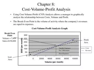
The Breakeven Graph • A standard breakeven graph has five components. • The horizontal axis (volume). • The vertical axis (dollars). • The fixed cost line. • The total cost line. • The total revenue line.
The Breakeven Graph • Normally, a loss area, profit area, and breakeven point will result. • At zero volume, net loss equals fixed costs.
0 200 600 400 Graphic Breakeven Analysis: Dakota Products, Inc. Total Revenue Line Net Income Area $60 Sales Breakeven $50 Total Cost Line $40 Variable Costs Dollars (in thousands) $30 Loss Area $20 Unit Breakeven Fixed Costs $10 Units of Output
Contribution Margin OBJECTIVE 6 Define contribution margin and use the concept to determine a company’s breakeven point for a single product and for multiple products.
Contribution Margin • Contribution margin equals sales minus total variable costs. CM = S - VC • Contribution margin per unit equals selling price minus variable cost per unit.
Contribution Margin • The breakeven point (in units) equals fixed costs divided by the contribution margin per unit. BE units = FC / CM per unit • A sales mix is used to calculate the breakeven point for each product when an organization sells more than one product.
Planning Future Sales OBJECTIVE 7 Apply cost-volume-profit analysis to estimated levels of future sales and to changes in costs and selling prices.
Cost-Volume-Profit • The contribution approach is extremely useful for profit planning. • Target sales in units = (FC + NI) / (CM per unit). • Projected net income can be calculated, assuming changes in volume, selling price, and/or costs.
Assumptions Underlying C-V-P Analysis 1. The behavior of variable and fixed costs can be measured accurately. 2. Costs and revenues have a close linear approximation. 3. Efficiency and productivity hold steady within the relevant range of activity.
Assumptions Underlying C-V-P Analysis 4. Cost and price variables hold steady during the period being planned. 5. The product sales mix does not change during the period being planned. 6. Production and sales volume are roughly equal.