Download
1 / 42
430 likes | 511 Views
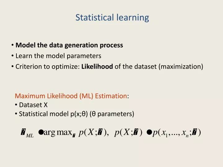
Statistical learning. Model the data generation process Learn the model parameters Criterion to optimize: Likelihood of the dataset (maximization). Maximum Likelihood (ML) Estimation : Dataset X Statistical model p(x; θ) ( θ parameters). Bayesian Learning.

E N D
Statistical learning • Model the data generation process • Learn the model parameters • Criterion to optimize: Likelihood of the dataset (maximization) • Maximum Likelihood (ML) Estimation: • Dataset X • Statistical model p(x;θ) (θ parameters)
Bayesian Learning Assign priors p(θ)on parameters of model p(x;θ) Priors: a flexible way to impose constraints on the model parameters. Bayesian learning: Given dataset X, compute posterior p(θ|Χ). MAP solution: It is possible that prior contains hyperparameters p(θ;λ).
p(h|f) p(f) p(g|h,f) Graphical Models • Graphical representation of the data generation process. • Represent dependenciesbetween random variables (r.v.) • Each node corresponds to one r.v. • Each directed edge denotes dependence of the rv at the end of edge from the rv in the beginning of the edge. p(g,h,f)=p(g|h,f)p(h|f)p(f)
Graphical Models • At each node i, the conditional probability p( Xi | pai ) is provided. • For directed acyclic graphs (Bayesian networks) it holds: • The model parameters θ exist in the conditional probabilities.
Graphical Models • Types of problems - Inference:compute distributions among RVs (joint, marginal, conditional) (use Bayes theorem and marginalization) • Parameter estimation - Combination of the above • Given a dataset, RVs are distinguished intoobserved andhidden (or latent).
Maximum Likelihood (ML) Estimation in Graphical models Dataset: Υ={y1,…,yn} (observations) Log-likelihood: Likelihood can defined bymarginalizinghidden RVs x: P(Y,X): complete likelihood
ΕΜ algorithm (Expectation-Maximization) • Iterative method for maximizing likelihood P(Y;Θ) (wrtΘ) when there existhidden variables x=(x1,…,xL). • Starting from a parameter vector Θ(0) , two steps at each iteration: • Ε-step: computer posterior P(x|Y;Θ(t)) (inference) • M-step: estimate Θ by maximizingexpectedcompletelog-likelihood: At each EM iteration the likelihood increases. Typically we terminate at local maximum. Strong dependence on initial parameters Θ(0). Expectedcompletelog-likelihood is easy to compute in some cases (e.g.mixture models). Problem: in several models the posterior P(x|Y;Θ) cannot be computed EM cannot be applied.
Gaussian distribution: x=(x1, …, xd)T : Mean μ=(μ1, …, μd)T , μ=Ε[x] Covariance matrix Σ Σ=Ε[(x-μ)(x- μ)T] (symmetric, positive definite) T = Σ-1(precision matrix) Models cloud-shaped data.
Cases for Σ • (a) Σ full • (b) Σ diagonal: • • statistical independenceamong xi • (c) Σ=σ2Ι (spherical):
Mixture models Mpdf componentsφj(x) Mixing weights: π1, π2, …, πM (priors) Data generation: • select a componenti (using priors) • sample from φi(x) Gaussian mixture models (GMMs): componentsφj(x) are Gaussian with θj=(μj, Σj)
GMMs can approximate an arbitrary pdf if the number of components becomes arbitrarily large. Posterior distribution: Can be used for clustering
EM for GMMs Dataset X={x1,…,xN}: M is given in advance Hidden variables:zi=(zi1,…,ziM): zij=1 xi has been generated byφj. GMMs can be trained through EM. ΕΜ applies easily since we can computer P(z=j|x).
EM for Mixture Models At each iteration t: E-βήμα: Compute the distributionof zij Define expected complete log-likelihood: M-βήμα: Update parameters
ΕΜ for GMMs M-stepforGaussian components (closed form solution): EM guarantees that:
Other Mixture Models • Mixture of multinomials (discrete data) • Mixture of Student-t (robust to outliers) • Regression mixture models (time series clustering) • Spatial mixture models (image segmentation)
Likelihood maximization: The variational approach Letxthe hidden RVs andY the observations in a graphical model. For everypdf q(x) it holds that: (Κullback-Leibler distance) F(Y;q,Θ) = Eq(ln p(Y,x;Θ))-Eq(lnq(x)): lower bound (variational bound) ofL(Υ;Θ). L(Y;Θ) ≥ F(Y;q,Θ) q(x): variational approximationofp(x|Y;Θ). Equality holds when q(x)=p(x|Y;Θ).
Variational ΕΜ (Neal & Hinton, 1998) Maximize the variational bound F(Y;q,Θ)wrtq and Θ, instead of maximizingL(Y;Θ)wrt Θ. VE-step: VM-step: The maximumof F(q,Θ)wrtq occurs forq(x)=P(x|Y;Θ) (thenVE-step ≡E-step, VM-step ≡ M-step ΕΜ algorithm). Whenp(x|Y) cannot be computed analytically, thenin theVE-step we use approximations that just increase F (without maximizingF).
Update q (VΕ-step): 1) Parametric form q(x;λ): parametersλare updated in E-step. 2)Mean field approximation Solution: Non-linear system of equations < >ki : expectation wrt allqk(xk), except forqi(xi)
Bayesian GMM Bayesian GMMs Priors on parameters θ: π, μ={μj}, Τ={Τj} whichbecome RVs Conjugate priors are selected: p(θ|Y) same form asp(θ).
Bayesian GMMs Priorp(μ) (almost uniform) discouragessolutionshaving GMM components in the same region (desirable feature). Prior p(T)=Wishart(v,V) discourages solutions with GMM components having covariance Σ very different from V (undesirable feature). Prior p(π)prevents redundant GMM components to be eliminated (undesirable feature).
Μπεϋζιανή μικτή κατανομή Variational learning of Bayesian GMMs MaximizeF wrtq (no model parameters θ to be learnt). Dataset Υ={yi} i=1,…,N. M components: N(μj, Tj), (j=1,…,M), π=(π1, π2,..., πΜ) Hidden RVs: x={xi}(i=1,…,N), π, μ={μj}, T={Tj}(j=1,…,M)
Variational learning of Bayesian GMMs (Attias, NIPS 1999): Mean field approximation q(x,π,μ,T)=q(x)q(θ): Non-linear System of equations for q(z)=q(x)q(θ). Solved using an iterative update method.
Variational learning of Bayesian GMMs In mixture models by setting some πi=0 we can change the model order (number of components) Prior p(π) prevents elimination of redundant components. Corduneanu & Bishop, AISTATS 2001: πiareconsidered as parameters and not RVs (Dirichlet prior on π is removed) Starting from a large number of components. We maximizeF(q(x,μ,Τ);π) wrt - q(x,μ,Τ) (VE-step) (mean field approximation) - π (VΜ-step) For the redundant components, VM-step update will give πj=0 (component i will be eliminated from GMM).
Unsupervised Dimensionality Reduction • Feature Extraction: new features are created by combining the original features • The new features are usually fewer than the original • No class labels available (unsupervised) • Purpose: • Avoid curse of dimensionality • Reduce amount of time and memory required by data mining algorithms • Allow data to be more easily visualized • May help to eliminate irrelevant features or reduce noise • Techniques • Principal Component Analysis (optimal linear approach) • Non-linear approaches (e.g. autoencoders, Kernel PCA)
Principal components: Vectors originating from the center of the dataset (data centering: use (x-m) instead of x, m=mean(X)) Principal component #1 points in the direction of the largest variance. Each subsequent principal component is orthogonal to the previous ones, and points in the directions of the largest variance of the residual subspace PCA: Principal Component Analysis
PCA algorithm • Given data {x1, …, xn}, compute covariance matrix : • PCA basis vectors = the eigenvectors of (dxd) • { i, ui }i=1..N = eigenvectors/eigenvalues of • 1 2 … d(eigenvalue ordering) • Select { i, ui }i=1..q (top q principal components) • Usually few λi are large and the remaining quite small • Larger eigenvalue more important eigenvectors • How to select q? : percentage of ‘explained variance’
PCA algorithm • W=[u1u2 … uq ]T (kxd projection matrix) • Z=X*WT (nxq data projections) • Xrec=Z*W (nxd reconstructions of X from Z) • PCA is optimal Linear Projection: minimizes the reconstruction error: • In autoencoders we also minimize the same criterion, but the model is non-linear.
PCA example: face analysis Original dataset: images 256x256
PCA example: face analysis Principal components: 25 top eigenfaces
PCA example: face analysis Reconstruction examples
z=(z1,…,zq) x=(x1,…,xd)
Probabilistic PCA: EM algorithm • E-step: • M-step: • Parameters W, σ should be initialized (randomly).