Download
1 / 40
420 likes | 1.21k Views
Definition and Properties of the Production Function. Lecture II. Overview of the Production Function.

E N D
Definition and Properties of the Production Function Lecture II
Overview of the Production Function • “The production function (and indeed all representations of technology) is a purely technical relationship that is void of economic content. Since economists are usually interested in studying economic phenomena, the technical aspects of production are interesting to economists only insofar as they impinge upon the behavior of economic agents.” (Chambers p. 7).
“Because the economist has no inherent interest in the production function, if it is possible to portray and to predict economic behavior accurately without direct examination of the production function, so much the better. This principle, which sets the tone for much of the following discussion, underlies the intense interest that recent developments in duality have aroused.” (Chambers p. 7).
A Brief Brush with Duality • The point of these two statements is that economists are not engineers and have no insights into why technologies take on any particular shape. • We are only interested in those properties that make the production function useful in economic analysis, or those properties that make the system solvable.
One approach would be to estimate a production function, say a Cobb-Douglas production function in two relevant inputs:
Given this production function, we could derive a cost function by minimizing the cost of the two inputs subject to some level of production:
Thus, in the end, we are left with a cost function that relates input prices and output levels to the cost of production based on the economic assumption of optimizing behavior. • Following Chamber’s critique, recent trends in economics skip the first stage of this analysis by assuming that producers know the general shape of the production function and select inputs optimally. Thus, economists only need to estimate the economic behavior in the cost function.
Following this approach, economists only need to know things about the production function that affect the feasibility and nature of this optimizing behavior. • In addition, production economics is typically linked to Sheppard’s Lemma that guarantees that we can recover the optimal input demand curves from this optimizing behavior.
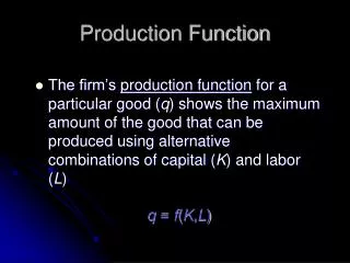
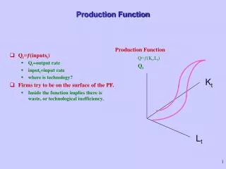
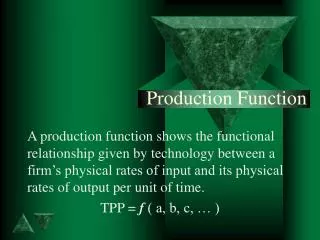
Production Function Defined • Following our previous discussion, we then define a production function as a mathematical mapping function:
However, we will now write it in implicit functional form This notation is sometimes referred to as a netput notation where we do not differentiate inputs or outputs.
Following the mapping notation, we typically exclude the possibility of negative outputs or inputs, but this is simply a convention. In addition, we typically exclude inputs that are not economically scarce such as sunlight. • Finally, I like to refer to the production function as an envelope implying that the production function characterizes the maximum amount of output that can be obtained from any combination of inputs.
Properties of the Production Function • Monotonicity and Strict Monotonicity:
The set V(y) is closed and nonempty for all y > 0. • f(x) is finite, nonnegative, real valued, and single valued for all nonnegative and finite x. • Continuity • f(x) is everywhere continuous; and • f(x) is everywhere twice-continuously differentiable.
Properties (1a) and (1b) require the production function to be non-decreasing in inputs, or that the marginal products be nonnegative. • In essence, these assumptions rule out stage III of the production process, or imply some kind of assumption of free-disposal. • One traditional assumption in this regard is that since it is irrational to operate in stage III, no producer will choose to operate there. Thus, if we take a dual approach (as developed above) stage III is irrelevant.
Properties (2a) and (2b) revolve around the notion of isoquants or as redeveloped here input requirement sets. • The input requirement set is defined as that set of inputs required to produce at least a given level of outputs, V(y). Other notation used to note the same concept are the level set.
Strictly speaking, assumption (2a) implies that we observe a diminishing rate of technical substitution, or that the isoquants are negatively sloping and convex with respect to the origin.
Assumption (2b) is both a stronger version of assumption (2a) and an extension. For example, if we choose both points to be on the same input requirement set, then the graphical depiction is simply
If we assume that the inputs are on two different input requirement sets, then Clearly, letting q approach zero yields f(x) approaches f(x*), however, because of the inequality, the left-hand side is less than the right hand side. Therefore, the marginal productivity is non-increasing and, given a strict inequality, is decreasing.
As noted by Chambers, this is an example of the law of diminishing marginal productivity that is actually assumed. • Chambers offers a similar proof on page 12, learn it.
The notion of weakly and strictly essential inputs is apparent. • The assumption of weakly essential inputs says that you cannot produce something out of nothing. Maybe a better way to put this is that if you can produce something without using any scarce resources, there is not an economic problem. • The assumption of strictly essential inputs is that in order to produce a positive quantity of outputs, you must use a positive quantity of all resources.
Different production functions have different assumptions on essential inputs. It is clear that the Cobb-Douglas form is an example of strictly essential resources.
The remaining assumptions are fairly technical assumptions for analysis. First, we assume that the input requirement set is closed and bounded. This implies that functional values for the input requirement set exist for all output levels (this is similar to the lexicographic preference structure from demand theory).
Also, it is important that the production function be finite (bounded) and real-valued (no imaginary solutions). The notion that the production function is a single valued map simply implies that any combination of inputs implies one and only one level of output.
Law of Variable Proportions • The assumption of continuous function levels, and first and second derivatives allows for a statement of the law of variable proportions. • The law of variable proportions is essentially restatement of the law of diminishing marginal returns.
The law of variable proportions states that if one input is successively increase at a constant rate with all other inputs held constant, the resulting additional product will first increase and then decrease. • This discussion actually follows our discussion of the factor elasticity from last lecture
Elasticity of Scale • The law of variable proportions was related to how output changed as you increased one input. Next, we want to consider how output changes as you increase all inputs.
In economic jargon, this is referred to as the elasticity of scale and is defined as
The elasticity of scale takes on three important values: • If the elasticity of scale is equal to 1, then the production surface can be characterized by constant returns to scale. Doubling all inputs doubles the output. • If the elasticity of scale is greater than 1, then the production surface can be characterized by increasing returns to scale. Doubling all inputs more than doubles the output.
Finally, if the elasticity of scale is less than 1, then the production surface can be characterized by decreasing returns to scale. Doubling all inputs does not double the output. • Note the equivalence of this concept to the definition of homogeneity of degree k: