Download
1 / 106
1.1k likes | 1.28k Views
CHAPTER 11 Output and Costs. The Firm’s Objectives and Constraints. The firm’s main objective is to maximize economic profits . This means they are making the best (most efficient) use of scarce resources.

E N D
The Firm’s Objectivesand Constraints • The firm’s main objective is to maximize economic profits. • This means they are making the best (most efficient) use of scarce resources. • Firms that try to maximize economic profits will have the best chance of surviving in a competitive environment.
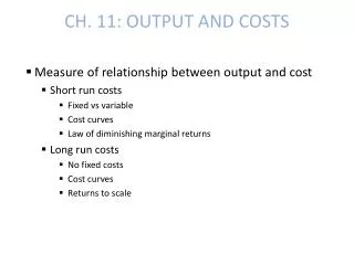
The Firm’s Objectiveand Constraints • The Short Run and the Long Run • The short run is a period of time in which the quantity of capital is fixed and the quantities of the other inputs (mainly labor) can be varied. • The long runis a period of time in which the quantities of all inputs can be varied.
How Long Is the Long Run? • In some industries — consulting or photocopying services — the short run may last only a month or two. • In other industries, the short run can be several years. Electric power generating and railroads are two industries that take years to build new capital.
Short-Run Technology Constraint • In order to increase outputin the short-run (holding the capital stock constant), firms must increase the quantity of labor.
Short-Run Technology Constraint • The effect of a change in the quantity of labor, holding the capital stock constant, can be described using three related concepts: • Total product is the total output produced. • Marginal product is the increase in total product that result from a one-unit increase in an input. • Average product is the total product divided by the quantity of inputs.
Total Product • Total product(TP) is the total quantity of output produced with a given quantity of a fixed input. • The total product curve shows the maximum quantity of output that can be produced with a given amount of capital as the amount of labor employed is varied.
The Total Product Curve • The total product curve is similar to the production possibilities frontier. • Both separate attainable output levels from those that are unattainable. • Only points on the total product curve are technologically efficient.
Total Product Schedule Labor Output a 0 0 b 14 c 2 10 d 3 13 e 4 15 f 5 16
Total Product Curve 15 Output (sweaters per day) 10 5 0 1 2 3 4 5 Labor (workers per day)
Total Product Curve 15 f e d Output (sweaters per day) 10 c 5 b a 0 1 2 3 4 5 Labor (workers per day)
Total Product Curve TP 15 f e d Output (sweaters per day) 10 c 5 b a 0 1 2 3 4 5 Labor (workers per day)
Total Product Curve TP 15 f e Unattainable d Output (sweaters per day) 10 c Attainable 5 b a 0 1 2 3 4 5 Labor (workers per day)
Marginal Product • The marginal productof an input is the increase in total product divided by the increase in the quantity of the input employed, when the quantity of all other inputs is constant.
Marginal Product of Labor • The marginal product of labor(MP) is the increase in total product divided by the increase in the quantity of labor employed, when the quantity of capital is constant. • MP= TP/ L
Marginal Product of Labor Schedule Labor Total Product Marginal product of Labor a 0 0 - b 1 4 c 2 10 d 3 13 e 4 15 f 5 16
Marginal Product of Labor Schedule Labor Total Product Marginal product of Labor a 0 0 - b 1 4 4 c 2 10 d 3 13 e 4 15 f 5 16
Marginal Product of Labor Schedule Labor Total Product Marginal product of Labor a 0 0 - b 1 4 4 c 2 10 6 d 3 13 e 4 15 f 5 16
Marginal Product of Labor Schedule Labor Total Product Marginal product of Labor a 0 0 - b 1 4 4 c 2 10 6 d 3 13 3 e 4 15 f 5 16
Marginal Product of Labor Schedule Labor Total Product Marginal product of Labor a 0 0 - b 1 4 4 c 2 10 6 d 3 13 3 e 4 15 2 f 5 16
Marginal Product of Labor Schedule Labor Total Product Marginal product of Labor a 0 0 - b 1 4 4 c 2 10 6 d 3 13 3 e 4 15 2 f 5 16 1
Marginal Product Curve • Marginal product is also measured by the slope of the total product curve. • Increasing marginal returns occur when the marginal product of an additional worker exceeds the marginal product of the previous worker.
Marginal Product Curve • Diminishing marginal returns • Occur when the marginal product of an additional worker is less than the marginal product of the previous worker • Law of diminishing returns • As a firm uses more of a variable input, with a given quantity of fixed inputs, the marginal product of the variable input eventually diminishes
Marginal Product Curve TP 15 6 d Output (sweaters per day) 13 Marginal product (sweaters per day per worker) 4 10 c 3 5 2 4 0 1 2 3 4 5 0 1 2 3 4 5 Labor (workers per day) Labor (workers per day)
Marginal Product Curve TP 15 6 d Output (sweaters per day) 13 Marginal product (sweaters per day per worker) 4 10 c 3 5 2 4 0 1 2 3 4 5 0 1 2 3 4 5 Labor (workers per day) Labor (workers per day)
Marginal Product Curve TP 15 6 d Output (sweaters per day) 13 Marginal product (sweaters per day per worker) 4 10 c 3 5 2 4 0 1 2 3 4 5 0 1 2 3 4 5 Labor (workers per day) Labor (workers per day)
Marginal Product Curve The red highlights the point of diminishing returns TP 15 6 d Output (sweaters per day) 13 Marginal product (sweaters per day per worker) 4 10 c 3 5 2 4 0 1 23 4 5 0 1 23 4 5 Labor (workers per day) Labor (workers per day)
Marginal Product Curve The red highlights the point of diminishing returns TP 15 6 d Output (sweaters per day) 13 Marginal product (sweaters per day per worker) 4 10 c 3 5 2 4 0 1 2 3 4 5 0 1 2 3 4 5 Labor (workers per day) Labor (workers per day)
Marginal Product Curve The red highlights the point of diminishing returns TP 15 6 d Output (sweaters per day) 13 Marginal product (sweaters per day per worker) 4 10 c 3 5 2 4 0 1 23 4 5 0 1 23 4 5 Labor (workers per day) Labor (workers per day)
Marginal Product Curve The red highlights the point of diminishing returns TP 15 6 d Output (sweaters per day) 13 Marginal product (sweaters per day per worker) 4 10 c 3 5 2 4 MP 0 1 23 4 5 0 1 23 4 5 Labor (workers per day) Labor (workers per day)
Average Product • The average productof an input is equal to total product divided by the quantity of the input employed. • Average product tells us how productive, on average, a factor of production is.
Average Product of Labor • The average product of laboris total product divided by the quantity of labor employed, when the quantity of capital is constant. • AP = TP/L
Average Product of Labor Schedule Labor Total Product Marginal Average Product Product of Labor of Labor a 0 0 - - b 1 4 4 c 2 10 6 d 3 13 3 e 4 15 2 f 5 16 1
Average Product of Labor Schedule Labor Total Product Marginal Average Product Product of Labor of Labor a 0 0 - - b 1 4 4 4 c 2 10 6 d 3 13 3 e 4 15 2 f 5 16 1
Average Product of Labor Schedule Labor Total Product Marginal Average Product Product of Labor of Labor a 0 0 - - b 1 4 4 4 c 2 10 6 5 d 3 13 3 e 4 15 2 f 5 16 1
Average Product of Labor Schedule Labor Total Product Marginal Average Product Product of Labor of Labor a 0 0 - - b 1 4 4 4 c 2 10 6 5 d 3 13 3 4.33 e 4 15 2 f 5 16 1
Average Product of Labor Schedule Labor Total Product Marginal Average Product Product of Labor of Labor a 0 0 - - b 1 4 4 4 c 2 10 6 5 d 3 13 3 4.33 e 4 15 2 3.75 f 5 16 1
Average Product of Labor Schedule Labor Total Product Marginal Average Product Product of Labor of Labor a 0 0 - - b 1 4 4 4 c 2 10 6 5 d 3 13 3 4.33 e 4 15 2 3.75 f 5 16 1 3.20
Average Product Curve What does the average product curve look like?
Average Product Curve 6 Average product & Marginal product (sweaters per day per worker) 4.33 4 3 2 0 1 2 3 4 5 Labor (workers per day)
Average Product Curve 6 c Average product & Marginal product (sweaters per day per worker) d 4.33 e 4 b f 3 2 0 1 2 3 4 5 Labor (workers per day)
Average Product Curve 6 c Average product & Marginal product (sweaters per day per worker) d 4.33 e 4 b f 3 AP 2 0 1 2 3 4 5 Labor (workers per day)
Average Product Curve Maximum average product 6 c Average product & Marginal product (sweaters per day per worker) d 4.33 e 4 b f 3 AP 2 MP 0 1 2 3 4 5 Labor (workers per day)
The Relationship Between Marginal and Average • When marginal product is above average product, average is rising — marginal is pulling average up. • When marginal product is below average product, average is falling — marginal is pulling average down. • Marginal product intersects average where average is at its maximum.
Marginal and Average Grade • The marginal grade is the grade you receive in this class. • Your average grade is your G.P.A. (grade point average). • If the grade you get in this class is higher than your G.P.A., it will pull your G.P.A. up. • If, on the other hand, ...
The Shapes of theProduct Curves • Total, marginal, and average product curves for different goods will still have similar shapes because almost every production process incorporates two features: • Increasing marginal returns initially • Diminishing marginal returns eventually
Increasing Marginal Returns • Increasing marginal returns occur when the marginal product of an additional worker exceeds the marginal product of the previous worker. • Increasing marginal returns will usually be the rule when the quantity of labor employed is low.
Diminishing Marginal Returns • Diminishing marginal returnsoccur when the marginal product of an additional worker is less than the marginal product of the previous worker. • All production processes eventually reach a point of diminishing marginal returns.
The Law ofDiminishing Returns • As a firm uses more of a variable input, with a given quantity of fixed inputs, the marginal product of the variable input eventually diminishes. • Because marginal product eventually diminishes, so does average product.
Short-Run Cost • To produce more output in the short run, a firm must employ more labor. • This will also increase its cost. • To produce more output, a firm must increase its costs.