Download
1 / 60
600 likes | 740 Views
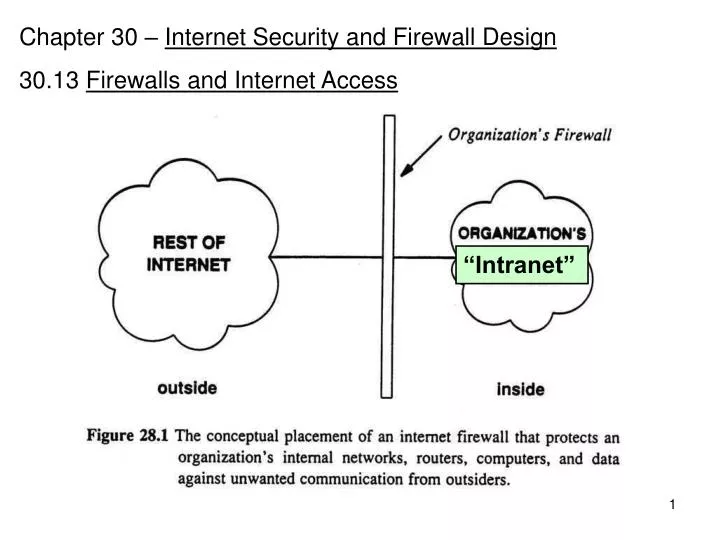
Chapter 30 – Internet Security and Firewall Design 30.13 Firewalls and Internet Access. “Intranet”. 30.13 Firewalls and Internet Access - continued Successful access control and content protection requires a careful combination of: ► restrictions on network topology

E N D
Chapter 30 – Internet Security and Firewall Design 30.13 Firewalls and Internet Access “Intranet”
30.13 Firewalls and Internet Access - continued Successful access control and content protection requires a careful combination of: ► restrictions on network topology ► intermediate information staging ► packet filters 30.14 Multiple Connections and Weakest Links Refers to first item above. In general, an organization’s intranet has multiple connections to the Internet. Must form a security perimeter by installing a firewall at each connection. All firewalls must be configured to have same access restrictions else entry through “weakest link.”
Chapter 30 – Internet Security and Firewall Design 30.13 Firewalls and Internet Access “Intranet”
Recall: ► restrictions on network topology ► intermediate information staging ► packet filters 30.15 Firewall Implementation and Packet Filters Refers to 3rd item. We have previously seen the addition of additional capability to a router – NAT. Now we add another capability – packet filter. Usually, a packet filter allows a manager to identify classes of datagrams by specifying arbitrary combinations of: ► source IP address ► destination IP address ► protocol ► source port ► destination port ► arrival interface
30.15 Firewall Implementation and Packet Filters- continued A packet filter is stateless; it treats each datagram in isolation, not “remembering” datagrams that arrived earlier and keeping no record of this event, apart from possibly writing to a log. We hope that the packet filter will operate at wire speed, not delaying incoming IP datagram traffic.
Recall row-by-row table search in routing: Figure 7.2
30.15 Firewall Implementation and Packet Filters - continued 128.5.0.0 When an IP datagram arrives, the packet filter will work through this table, row by row. If the datagram matches the specification on any row, the datagram will be filtered/blocked/discarded. The ports are not in the IP datagram header, so modified router must “drill down” into data.
Transport Like NAPT, packet filtering gets router involved in layer 4! (looking inside “data” in IP datagram, not just header)
30.16 Security and Packet Filter Specification This packet filter has specified a small list of services to be blocked. This does not work well, because: ► the number of well-known (i.e. server) ports is large and growing ► some Internet traffic does not travel to or from the well-known ports (e.g. organization can run WWW server on port 8080, instead of 80) ► listing ports of well-known services leaves the firewall vulnerable to tunneling (needs inside accomplice). This suggests reversing the idea of the filter: Instead of specifying types of datagram that should be filtered, specify types that should be forwarded. Everything else is filtered.
30.17 Consequences of Restricted Access for Clients Problemwith this scheme: It prevents a client inside the firewall from receiving a reply from a server outside the firewall. Why? Because the client chooses a source port at random, in the range 1024 to 65,536. In the server’s reply the client’s source port becomes the destination port. The packet filter would have to be configured to forward all of these possibilities.
30.18 Stateful Firewalls Recall that basic packet filters are stateless. They treat each IP datagram separately and keep no record of datagrams received. Stateful firewallswatch outgoing requests and adapt the filter rules to accommodate the replies. Example: Internal client sends TCP connection request to external WWW server. Stateful firewall records this as the two endpoints of the requested connection: ( IPsource, Portsource, IPdest, 80 ) When the server returns a connection accept the firewall will recognize this as a response to the request, and forward it to the client. This is additional to the packet filter, so actions can still be prohibited, as determined by the administrator.
30.18 Stateful Firewalls – continued In the previous example, what if no reply is received to the connection request after a reasonable time? The record of the connection must be purged – “soft state” How does the stateful firewall know when a TCP connection is terminated, so that the record can be deleted? Firewall must watch for the two FIN segments (“connection monitoring”)
Figure 12.15 Basically, the firewall must be following this state-transition diagram for each of the active connections!
30.19 Content Protection and Proxies Recall that successful access control requires a careful combination of: ► restrictions on network topology ► intermediate information staging ► packet filters Proxies refer to the second item. We have been concentrating on access, but we may also have to protect content. This is almost impossible at the packet-filter level, since content can be divided among many datagrams, which can arrive in any order and may be fragmented. The firewall must mimic the ultimate destination host by assembling the entire message for inspection – application proxy. This is going far beyond the original idea of a wire-speed firewall!
30.19 Content Protection and Proxies - continued PROXY “Transparent” proxy – apart from delay, client/user is unaware that there is a proxy. “Non-transparent” – client is configured to access proxy when it tries to access the external server.
30.20 Monitoring and Logging If you’re the network administrator, do it! Or else you don’t know what’s happening.
Background to Chapter 13 - 15 7.11 Establishing Routing Tables For now, assume routing tables are loaded manually; In chapters 13 and 15 we’ll see protocols that allow routers to learn routes from each other. End of Chapter 7.
BHM * ATL
8.11 Route Change Requests from Routers – continued This is not a general mechanism for route changes. It is restricted to routers sending to directly-connected hosts. Figure 8.7 – R5 cannot redirect R1 to use the shorter path from S to D But R1 could tell S to use R6 for traffic toD, provided that R6 is in R1’s routing table as “next hop” for destination D
13.6 Automatic Route Propagation “Routing protocols serve two important functions. First, they compute a set of shortest paths. Second, they respond to network failures or topology changes by continually updating the routing information.” A network administrator cannot respond manually to failures fast enough. 13.7 Distance Vector (Bellman-Ford) Routing This is the first type of automatic routing protocol that we shall study. At start-up routing tables include only the directly-connected networks. Figure 13.3
Figure 13.3 “Distance” for direct connection has been changed from 0 to 1 to agree with chapter 15. Routers advertise their capabilities to their directly-connected neighbors, using IP local broadcast capability.
13.7 Distance Vector (Bellman-Ford) Routing - continued Periodically, routers broadcast copies of their routing tables to all directly-connected routers. Consider router J sending to router K. We think of J as advertising “I can get you to network X at a cost of Y” “cost” means the number of routers along the path to X (router J plus subsequent routers). Router K will update its routing table on the basis of the information received from J.
Router K’s initial routing table To see how it works, assume that at some later time router K has learned routes and its routing table looks like this: Routers J, L, M, and Q are directly-reachable from K
Router K now receives an update message from directly-connected router J Recall that J says “I can get you to network X at a cost of Y” Router K’s routing table Update message from J Update items marked with arrow cause K to change its routing table.
Router K’s routing table Update message from J Resulting Changes to K’s routing table: ► to Net 4 – distance 4 – via J (a better route has been discovered) ► to Net 21 – distance 5 – via J (a new route has been discovered) ► to Net 42 – distance 4 – via J (something has gone wrong with the old route beyond J ) K will now advertise “I can get you to Net 4 at a cost of 4 via J” “I can get you to Net 21 at a cost of 5 via J” “I can get you to Net 42 at a cost of 4 via J”
13.7 Distance Vector (Bellman-Ford) Routing – continued Advantages: ► Distance-vector algorithms are easy to implement. ► In a relatively static environment they compute the shortest paths and propagate correct routes to all destinations. Disadvantages: ► All routers must participate ► In a large internet the update messages get large (size is proportional to the number of networks in the internet, so distance-vector algorithms “do not scale well”) ► When routes change rapidly the computations may not stabilize (changes propagate slowly – diffusion)
13.9 Link-State SPF) Routing An alternative to distance-vector routing is link-state routing. These are known as Shortest Path First (a misnomer, since all routing algorithms compute the shortest path) Every router has a graph (CS 250/350) showing all other routers and the networks to which they connect. Nodes in the graph are the routers; links in the graph are direct connections between routers. Periodically each router tests the reachability of all directly-connected routers (i.e. tests whether each of its links is “up” or “down”) The router multicasts this information to all other routers. If a receiving router detects a change in link status, the router recomputes shortest paths to all possible destinations, using Dijkstra’s algorithm.
Link-State Routing. Advantages: ► size of the update messages sent by a router is proportional to the number of links it has (i.e. update messages are much smaller than those in vector-distance, so link-state “scales better”) ► each router computes routes independently from original data (not relying on intermediate routers) Disadvantages: ► computational load on routers.
14.5 Autonomous System Concept We cannot run an automatic routing protocol for the entire Global Internet. How should the Internet be partitioned into sets of routers so that each set can run a routing update protocol? Networks and routers are owned by organizations and individuals. Within each, an administrative authority can guarantee that internal routes remain consistent and viable. For purposes of routing, a group of networks controlled by a single administrative authority is called an autonomous system (AS) identified by an autonomous system number. Comer suggests thinking about an autonomous system as corresponding to a large ISP (but UAB is an AS, number 3452)
One router can be chosen to inform the outside world of networks within the organization (assume desire for universal connectivity - temporarily ignore security!) This router also learns about outside networks and distributes this information internally.
14.6 Exterior Gateway Protocols and Reachability Figure 14.2 Within an autonomous system, the administration chooses a routing method. Between autonomous systems, the Border Gateway Protocol (BGP-4) is used. R1 gathers information about networks in AS1 and BGPs the info to R2 R2 gathers information about networks in AS2 and BGPs the info to R1.
Chapter 15: Routing Within an Autonomous System (RIP, OFPF) 15.3 Routing Information Protocol RIP is a straightforward implementation of distance-vector routing. Routers run RIP in “active mode,” broadcast update messages to directly-connected neighbors every 30 seconds. Hosts listen and learn, but do not broadcast.
15.3 Routing Information Protocol – continued RIP rules: ► routers send updates every 30 seconds ► receiving routers do not replace an existing route with one of equal cost (hop count) ► the maximum hop count is 16 (“infinity”) ► receivers use 180-second timeout on entries (“soft state”) We will use fig 15.2 to illustrate how RIP works.
Initially: R5 not running Other routers have only direct connections. N1 1 dir N2 1 dir N2 1 dir N3 1 dir N2 1 dir N3 1 dir N1 2 R1 N1 2 R1 N3 1 dir N4 1 dir N1 3 R2 N2 2 R2 N1 3 R5 N2 2 R5
15.4 Slow Convergence Problem Fig 15.4 (a)
R1 Fails! N1 1 N1 16 Send to R2 N1 3 R2 N1 3 N1 5 R2 N1 5 At this point we have a routing loop! N1 2 R1 N1 2 R2 N1 4 R1 N1 4 Send to R1 and R3 N1 6 R1 N1 6
15.4 Slow Convergence Problem Fig 15.4
15.5 Solving the Slow Convergence Problem Problem arises from sending back a route to the router that sent it. “Split horizon updates” prevent this. Easy to implement: recall figure 13.4: Router K’s routing table Router K must not send routes to Net 24 and Net 42 back to router J This is done in RIPv2
15.5 Solving the Slow Convergence Problem – continued Other techniques: after receipt of information that a network is unreachable: ► “hold down” ignore further information about that network for hold-down period (60 seconds) ► “poison reverse” with “triggered updates” continue to advertise path to that network, with cost 16 send immediate special update – don’t wait for the regular 30-second schedule.
15.9 RIP2 Extensions and Message Format Figure 15.6 COMMAND: 1 = request, 2 = response Route to Network 1 Goes next to this D-C router And this is the total distance to the destination over this route.
15.9 RIP2 Extensions and Message Format – continued In RIPv1 routers broadcast their messages, so that every computer in the local network had to process the message. This is wasteful. RIPv2 makes use of multicasting to the class–D “RIP2 routers” address 224.0.0.9. This sends messages specifically (only) to routers on the local network.
15.9 RIP2 Extensions and Message Format – continued RIP messages travel encapsulated in UDP datagrams Both source and destination ports are 520 (not client/server). 15.10 The Disadvantage of RIP Hop Counts Using hop counts as a metric does not always yield routes with the least delay or the highest capacity.
15.11 Delay Metric HELLO protocol measures delay of competing routes and selects route with least delay. 15.12 Delay Metrics and Oscillation HELLO is susceptible to oscillation between two routes with similar delay.
15.15 The Open SPF Protocol (OSPF) An Implementation of link-state routing. Features: ► open standard (not proprietary) ► type-of-service routing ► load balancing – “if a manager specifies multiple routes to a given destination at the same cost, OSPF distributes traffic over all routes equally.” ► can partition internets into areas ► exchanges between routers can be authenticated ► supports host-specific, subnet-specific, classful and class-less routes
15.16 Routing with Partial Information “Routers at the center of the Internet have a complete set of routes to all possible destinations; such routers do not use default routes.” (288,000 entries in routing tables in 2009 +14% /year) Most other routers do not have complete information they use default routes.
15.16 Routing with Partial Information - continued Using default routes for most routers has two consequences: ► local routing errors can go undetected – one router’s default may send datagrams to the wrong next-hop router (perhaps outside the autonomous system), but that router may quietly forward the datagram to the correct next hop (perhaps back inside the autonomous system); ► routing update messages exchanged by routers can be much smaller than if the messages contained all possible destinations (our original motivation for using default routes).
N3 2 R3 Sub-optimal routing No N3 Default R1
Lab Session 5 – Packet Filtering 1. Physical Connections Packet filter INSIDE: as usual (192.168.1.0) OUTSIDE: UAB class B address 138. 26. 0. 0 CIS subnet 138. 26. 66. 0 mask 255. 255. 255. 0 we will subnet further 255. 255. 255. 240