We’ll consider here the problem of paired data. There are two common notations.

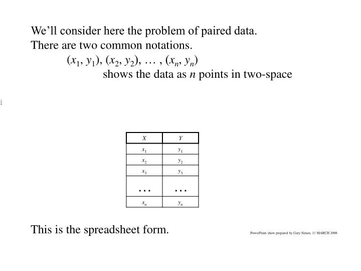
1. We’ll consider here the problem of paired data. There are two common notations. (x1, y1), (x2, y2), … , (xn, yn) shows the data as n points in two-space This is the spreadsheet form. PowerPoint show prepared by Gary Simon, 11 MARCH 2008.

2. The separate points are assumed independent. We wish to find a relationship between variable X and variable Y. We have here a data set on eye response to different types of drops, but for now we’ll look at just a few simple items of information. DP0OD Pupil diameter, start of experiment, right eye DP0OS Pupil diameter, start of experiment, left eye AGE Subject age There are altogether 100 subjects.

3. Let’s consider the relationship between pupil diameter in the eyes. An obvious first step is making a scatterplot showing all 100 people. Let’s put the right eye on the horizontal axis and the left eye on the vertical axis. This is not a critical decision. This graph shows that the points cluster near a diagonal line. This is not a surprise.

4. Here’s the same picture with the Y = X line superimposed: The points cling close to the line.

5. There are a few simple ways to summarize this situation. Perhaps the best is the correlation. Here r = 0.96. Now let’s complicate this a bit. Suppose that we want to check on the relationship between DP0OS (pupil diameter, left eye) and AGE.

6. These two variables are not symmetric. We’ll think of the variable AGE as “logically earlier.” This means that we obtain it easily, reliably, and (probably) earlier than the pupil diameter. Also, it’s logical to think of using AGE to predict pupil diameter. We will designate AGE as the independent variable, we will identify it with the symbol X, and we will place it on the horizontal axis of the coming scatterplot.

7. We’ll think of the variable DP0OS as “logically later.” This information is obtained with some difficulty, with possible error measurement, and (probably) later than the age. We will designate DP0OS as the dependent variable, we will identify it with the symbol Y, and we will place it on the vertical axis of the coming scatterplot.

8. The scatterplot is next. Before it’s shown, we should ask ourselves whether * pupil diameter generally rises with age * pupil diameter is unrelated to age * pupil diameter generally decreases with age What do you think?

9. Here is the scatterplot:

10. Suppose that you would like to summarize the relationship between the two variables. You would like to write Pupil Diameter = Y = dependent variable = f(AGE) = f(X) = f(independent variable) for some function f . The problem is that you’ll never find a believable function to go through all the dots on the scatterplot. There is too much statistical noise.

11. The expression of the model will be revised to Y = f(X) + ε The symbol ε represents statistical noise. It may involve random errors in measuring Y or it may just represent variability that we just don’t know to account for. One could also have made “multiplicative noise” in the form Y = f(X) × ε. In some cases, this is useful. For now, we’ll stick with the “additive noise” with the + sign. We will have a lot to say about the ε term. For now, we’ll just assume that it is independent over the data points.

12. What form should we use for the function f ? How about f(X) = log X ? How about f(X) = a X2 + b X + c ? How about f(X) = tan( a X2 + h) ? How about f(X) = ?

13. We will start with the simplest function, the straight line. This is f(X) = β0 + β1X . The symbols β0 and β1 are parameters. β0 is the intercept, also called Y-intercept. β1 is the slope. In nearly all cases, β0 and β1 are not known, and we have to estimate them from data.

14. The notation is not universal. You will also see f(X) = α + βX This is OK. f(X) = a + bX Use of Roman letters is not recommended. For issues related to considering which symbols are fixed and which are random, we will prefer f(x) = β0 + β1x . That is, we will prefer lower-case x. It is however impossible to enforce distinctions between x and X and also between y and Y. We can’t be too dogmatic about the notation.

15. The relationship between Y and X will be described through the simple linear regression model Y = β0 + β1x + ε This is made more direct by putting on subscript i to label individual data points. Our preferred form for the simple linear regression model is Yi = β0 + β1xi + εi with i = 1, 2, …, n.

16. The simple linear regression model also includes these assumptions about the noise terms ε1 , ε2 , ε3 , … , εn : The ε’s are independent of each other and also independent of the x’s. The ε’s are sampled from a hypothetical population in which the mean is zero and the standard deviation is σ. In some cases, we may add in the further assumption that the ε’s are sampled from a normal population.

17. The simple linear regression model Yi = β0 + β1xi + εi has three unknown parameters: β0 , β1 , and σ . Estimating these parameters is an important part of the regression task. Estimating β0 and β1 is equivalent to drawing a line on the scatterplot. The estimate of σ tells us how well the line describes the set of points on the scatterplot.

18. The estimate of β0 is written b0 . The estimate of β1 is written b1 . The estimate of σ is written s . You’ll also see sεor sY | x . Note this consistent pattern of usage: Model parameters are Greek letters. Data-based estimates are corresponding Latin letters.

19. Be aware that other schemes exist. Someone who writes the model as Yi = α + βxi + εiwill use a for the estimate of α and will use b for the estimate of β. Someone who writes the model as Yi = a + b xi + εi will use for the estimate of a and will use for the estimate of b.

20. For our problem, the model is DPi = β0 + β1 AGEi + εi The pupil diameter DP is in units of mm (millimeters). The variable AGE is in units of years. Therefore, β0 and its estimate b0 are in units of mm. Also, the ε’s and their standard deviation σ are in units of mm. The estimate of σ is also in units of mm. The slope β1 and its estimate b1 are in units of .

21. How should we estimate β0 and β1 ? We could guess. We could draw a nice-looking line on the scatterplot and then use that line to get the estimates. These are not necessarily bad methods, but they are not reproducible. This means that different people get different answers. Worse yet, the same person on two occasions will produce different answers.

22. We will instead propose that the estimates be done by minimizing a mathematical function. Many proposals have been made, but the nearly universal choice is least squares. Choose b0 and b1 to minimize the function Q = How should this minimization be done?

23. The solution is by (mindless and routine) differentiation. That is, solve the system This results in two linear equations in the two unknowns b0 and b1 .

24. The solution method selected by the previous slide works, but it’s clumsy. Here is a cleaner way to do this. • Find the five sums , , • , , . • Next find these quantities: • , , Sxx = , • Syy = , Sxy =

25. (3) Find b1 (the estimate of the slope β1) as b1 = • Find b0 (the estimate of the intercept β0) as • b0 = - b1 Note that b1 is found before b0 .

26. Finally, calculate • Syy | x = We’ll use this later in the estimation of σ, the standard deviation of the noise.

27. While it’s possible to do this for our problem of pupil diameter versus age with just the use of a calculator… there are too many steps and we are likely to make errors. We’ll give this to the Minitab function Stat > Regression > Regression.

28. The Minitab output is extensive, but from it we find Regression Analysis: DP0OD versus AGE The regression equation is DP0OD = 7.27 - 0.0430 AGE This is called the fitted regression equation. This identifies for us b0 = 7.27 and b1 = -0.0430.

29. Here is a reprise of the scatterplot, now shown with the fitted regression line. This was made in Minitab with Stat > Regression > Fitted Line Plot. This has reported also sε = 0.832776, the estimate of σ.

30. It’s important to distinguish population quantities from sample quantities. The process of regression is not simply “numbers in”  “numbers out.”

31. The simple linear regression model is Yi = β0 + β1xi + εi If you are asked to graph the line Y = β0 + β1x . . . Please refuse! You cannot graph this line because β0 and β1 are unknown population parameters.

32. With data, you will get the estimates b0 and b1. The fitted regression line is = b0 + b1x . The “hat” on is helpful, but it’s a typesetting nuisance. The fitted line is often given without the “hat.”

33. For the pupil diameter problem, the fitted line is = 7.27 - 0.0430 AGE The interpretation of -0.0430 is . . . that each year of age is associated with a reduction of 0.0430 mm in pupil diameter. The interpretation of 7.27 is . . . to be avoided. It’s tempting to say that it’s an assessment of pupil diameter at birth. The data set did not have anyone younger than 18, so we won’t force an interpretation.

34. The estimate of the noise standard deviation was calculated as sε = 0.832776. This is about 0.83 mm, which is rather large for this context. What are we to make of this large value? This is saying that AGE is far from a perfect predictor of pupil diameter.

35. We still have to decide * Is there an objective way to decide if this whole activity was worth doing? * Is there an objective way to decide if the model Yi = β0 + β1xi + εi was a good choice?