Download
1 / 43
450 likes | 725 Views
Basic Population Genetics and One and Two locus models of Selection. Given genotype frequencies, we can always compute allele frequencies, e.g.,. X. 1. p. =. f. r. e. q. (. A. ). =. f. r. e. q. (. A. A. ). +. f. r. e. q. (. A. A. ). i. i. i. i. i. j. 2. i. 6.

E N D
Basic Population Geneticsand One and Two locus models of Selection
Given genotype frequencies, we can always compute allele frequencies, e.g., X 1 p = f r e q ( A ) = f r e q ( A A ) + f r e q ( A A ) i i i i i j 2 i 6 j = Ω 2 p f o r i = j i f r e q ( A A ) = i j 2 p p f o r i = 6 j i j Allele and Genotype Frequencies The converse is not true: given allele frequencies we cannot uniquely determine the genotype frequencies For n alleles, there are n(n+1)/2 genotypes If we are willing to assume random mating, Hardy-Weinberg proportions
Hardy-Weinberg • Prediction of genotype frequencies from allele freqs • Allele frequencies remain unchanged over generations, provided: • Infinite population size (no genetic drift) • No mutation • No selection • No migration • Under HW conditions, a single generation of random mating gives genotype frequencies in Hardy-Weinberg proportions, and they remain forever in these proportions
f r e q ( A A B B ) = f r e q ( A B j f a t h e r ) f r e q ( A B j m o t h e r ) f r e q ( A a B B ) = f r e q ( A B j f a t h e r ) f r e q ( a B j m o t h e r ) + f r e q ( a B j f a t h e r ) f r e q ( A B j m o t h e r ) Gametes and Gamete Frequencies When we consider two (or more) loci, we follow gametes Under random mating, gametes combine at random, e.g. Major complication: Even under HW conditions, gamete frequencies can change over time
ab AB AB ab AB ab AB ab In the F1, 50% AB gametes 50 % ab gametes If A and B are unlinked, the F2 gamete frequencies are AB 25% ab 25% Ab 25% aB 25% Thus, even under HW conditions, gamete frequencies change
f r e q ( A B ) = f r e q ( A ) f r e q ( B ) f r e q ( A B C ) = f r e q ( A ) f r e q ( B ) f r e q ( C ) f r e q ( A B ) 6 = f r e q ( A ) f r e q ( B ) D = f r e q ( A B ) ° f r e q ( A ) f r e q ( B ) A B Linkage disequilibrium Random mating and recombination eventually changes gamete frequencies so that they are in linkage equilibrium (LE). Once in LE, gamete frequencies do not change (unless acted on by other forces) At LE, alleles in gametes are independentof each other: When linkage disequilibrium (LD) present, alleles are no longer independent --- knowing that one allele is in the gamete provides information on alleles at other loci The disequilibrium between alleles A and B is given by
f r e q ( A B ) = f r e q ( A ) f r e q ( B ) + D A B Departure from LE LE value t D ( t ) = D ( 0 ) ( 1 ° c ) Initial LD value The Decay of Linkage Disequilibrium The frequency of the AB gamete is given by If recombination frequency between the A and B loci is c, the disequilibrium in generation t is Note that D(t) -> zero, although the approach can be slow when c is very small
Key Points Under HW changes in allele frequencies are permanent Changes due to LD are transient, and decay away on their own Implications for trait selection: Changes in allele frequencies produce permanent change Changes in genotype frequencies induced by selection that are out of HW decay back to HW (at new allele frequencies) when selection stops.
Genetic Drift Random sampling of 2N gametes to form the N individuals making up the next generation results in changes in allele frequencies. This process, originally explored by Wright and Fisher, is called Genetic Drift. Suppose there are currently i copies of allele A, so that freq(A) = p = i/(2N) That probability that, following a generation of random sampling, the freq of A is j/(2N) is
- - µ ∂ µ ∂ ( ) ( ) j N ° j N ! i N ° i P r ( i c o p i e s ! j c o p i e s ) = - ( N ° j ) ! j ! N N This probability follows binominal sampling, Hence, if the current allele frequency is p, the expected allele frequency in the next generation is also p, but with sampling variance p(1-p)/(2N) Thus, with N is large, the changes in allele frequency over any generate are expected to be rather small However, the cumulative effects of generations of such sampling are very considerable.
Eventually, any random allele will either be lost from the population or fixed. If the allele has initial frequency p, then Pr(Fixation) = p Pr(loss) = 1- p The expected time to fixation is on order of 4N generations. If selection is sufficiently weak, it can be overpowered by drift.
Single-locus selection The basic building block is a single locus under selection. Think of this as a trait controlled by only a single gene Individuals differ in fitness when they leave different numbers of offspring When the fitness of at least one genotype is different from the others, selection occurs
W W W W = p2 WAA + 2p(1-p) WAa + (1-p)2Waa Where is the mean population fitness, the fitness of an random individual, e.g. = E[W] One locus with two alleles W
- - 2 p W + p ( 1 ° p ) W p W + ( 1 ° p ) W A A A a A A A a 0 p = = p W W The new frequency p’ of A is just freq(AA after selection) + (1/2) freq(Aa after selection) The fitness rankings determine the ultimate fate of an allele If WXX> WXx > Wxx, allele X is fixed, x lost If WXx > WXX, Wxx, selection maintains both X & x Overdominant selection
Class problem Equations 5.3c-5.3d in notes given approximate expressions for the time to change from frequency p0 to p Compute the time to change from frequency 0.1 to 0.9 Fitness are 1 : 1.01: 1.02 Fitness are 1: 1:02: 1.02 Fitness are 1: 1: 1.02
Wright’s formula Computes the change in allele frequency as as function of the change in mean fitness Requires frequency-independence: Genotype fitnesses are independent of genotype frequencies, d Wij / pi = 0 Note sign of change in p = sign of dW/dp
Key: Internal equilibrium frequency. Stable equilibrium Application: Overdominant selection
A common model for stabilizing selection on a trait is to use a normal-type curve for trait fitness Application: Stabilizing selection As detailed in Example 5.6, we can use Wright’s formula to compute allele frequency change under this type of selection This is selective underdominance! If p < 1/2, Dp <0 and allele gets lost. If p > 1/2, Dp > 0 and allele fixed. Hence, stabilizing selection on a trait controlled by many loci removes variation!
n n X X W i 0 p = p ; W = p W ; W = p W Wi = marginal fitness of allele Ai i i j i j i i i W j = 1 i = 1 W = mean population fitess = E[Wi] = E[Wij] If Wi > W, allele Ai increases in frequency If a selective equilibrium exists, then Wi = W for all segregating alleles. Multiple Alleles Let pi = freq(Ai), Wij = fitness AiAj
Consider average excess in relative fitness for Ai Allele frequency change is a function of the average excess of that allele Fitness as the ultimate quantitative trait Recall that the average excess of allele Ai is mean trait value in Ai carries minus the population mean Allele frequency does not change when its average excess is zero At an equilibrium, all average excesses are zero. Hence, no variation in average excesses and thus no additive variation in fitness at equilibrium
Wright’s formula with multiple alleles Key: Note that the sign of dW/dpi does not determine sign(Dp). Thus an allele can change in a direction opposite to that favored by selection if the changes on the other alleles improve fitness more Prelude to the multivariate breeder’s equation, R = Gb
General features with multiple allele selection With Wij constant and random mating, mean fitness always increases What about polymorphic equlibrium? Require Wi = W1 for all i. Kingman showed there are only either zero, one, or infinitely many sets of equilibrium frequencies for an internal equilibrium
Equilibrium behavior Single internal equilibrium if W has exactly one positive and at least one negative, eigenvalue e an eigenvalue of W if We = le Other equilibrium can potentially fall anywhere on the simplex of allele frequencies
When two (or more) loci are under selection, single locus theory no longer holds, because of linkage disequilibrium (i.e., freq(ab) = freq(a)*freq(b) Two-locus selection Consider the marginal fitness of the AA genotype Note that this is a function of p = freq(A), q=freq(B), and D = freq(AB)-p*q. When D = 0 this reduces to Here, W(AA) is independent of freq(A) = p, and we can use Wright’s formula to compute allele frequency change.
For two loci, follow gametes The resulting recursion equations, even for the simple two biallelic loci, do not have a general solution for their dynamics When selection is strong and linkage (c) tight, results can be unpredictable Mean fitness can decline under two-locus selection
At equilibrium If LD at equilibrium, the second term is nonzero and not all gametes have the same marginal fitness. Note that when c=0, this is just a 4 allele model, and all segregating alleles have the same marginal fitness If equilibrium LD is not zero, mean fitness is not at a local maximum. However, unless c is very small, it is usually close In such cases, mean fitness decreases during the final approach to the equilirium (again, effects usually small)
Note complete additivity in the trait. W(z) = 1 - s(z-2)2 Fitness function induces dominance and epistasis for a completely additive trait At equilibrium, no additive variance in FITNESS -- still could have lots of additive variance in the trait. Example 5.11. Even apparently simple models can have complex behavior.
FFT: Fisher’s Fundamental Theorem What, in general can be said above the behavior of multilocus systems under selection? Other than they are complex, no general statement! Some rough rules arise under certain generalizations, such as weak selection -- weak selection on each individual locus, selection on the trait could be strong. One such rule, widely abused, is Fisher’s Fundamental theorem Karlin: “FFT is neither fundamental nor a theorem”
Fisher: “The rate of increase in fitness of any organism at any time is equal to its genetic variance in fitness at that time” Classical Interpretation: D Wbar = VarA(fitness) This interpretation holds exactly only under restricted conditions, but is often a good approximate descriptor For example, approximately true under weak selection Important corollary holds under very general conditions: in the absence of new variation from mutation or other sources such as migration, selection is expected to eventually remove all additive genetic variation in fitness
Additive variance in fitness is key. Consider a selective overdominant locus, 1:1+s:1. Maximal total genetic variance occurs at p =1/2, but heritability is zero at this value, and hence no response to selection Generally, traits associated with fitness components (e.g., viability, # offspring) have lower h2 and also more non-additive variance.
Traits more closely associated (phenotypically correlated) with fitness had lower heritabilities in Collared flycatchers (Ficedula albicollis) on the island of Gotland in the Baltic sea, (Gustafsson 1986)
Lack of such associated (fitness measure by seed production) for Plox ( Phlox drummondii) in Texas (Schwaegerle and Levin 1991). Again, phenotypic correlated used.
Life history and morphological traits in the Scottish red deer ( Cervus elaphus). Circles denote life-history traits, squares morphological traits. Genetic correlation between trait and fitness (Kruuk et al. 2000)
Houle: Evolvability Traits are generalized standardized to compare them with others: Common is variance standarization, x’ = x/sx On such a scale, a response (change in mean) of 0.1 implies a 0.1 standard-deviation change in the mean. variance-standardization thus a function of standing variation in the population. Houle agreed that our interest is typically in the proportion of change -- e.g, animals are 5% larger. A 0.1 response on this scale means the trait improved by 10% This uses mean standardization, x’ = x/m Houle said that evolvability of a trait, sA/m is a better measure of evolutionary potential than h2 = sA2 / sz2 Houle found that life history traits had HIGHER evolvabilities. They had more genetic variation, but also more environmental variance, resulting in lower h2
CVA = Genetic Coefficient of variation: CVA2 = Var(A)/mean2 Life history and morphological traits in the Scottish red deer ( Cervus elaphus). Circles denote life-history traits, squares morphological traits. Genetic correlation between trait and fitness (Kruuk et al. 2000)
Robertson’s secondary theorem and the breeder’s equation FFT under weak selection gives some approximate rules about how populations evolve by following changes in fitness Response = change in mean equals the additive genetic covariance between trait and fitness (the covariance within an individual for the breeding values of these two traits). With weak selection, we can use population-genetic models based on Robertson’s idea to express response in terms of gene frequency changes Alan Robertson proposed a ``secondary theorem” to Fisher’s to treat trait evolution, We are usually much more interest in changes in trait values. What can we say here? More generally, when there is selection to change the variance as well (ds) If no dominance, d =0, and R = h2S However, if there is skew in the phenotype, and skew in the breeding values, then breeder’s equation does not exactly hold If selection only on mean and no skew, ds= -S and we recover Breeders, R = h2S
1 ° e x p ( ° 4 N s p ) U ( p ) = 1 ° e x p ( ° 4 N s ) Selection and Drift If the strength of selection is weak relative to the effects of drift, drift will overcome the directional effects of selection. Suppose genotypes AA : Aa : aa have fitnesses 1 + 2s : 1 + s : 1 Kimura (1957) showed that the probability U(p) that A is fixed given it starts with frequency p is
Note if 4Ns >> 1, allele A has a very high probability of fixation If 4Ns << -1 (i.e. allele is selected against), A has essentially a zero probability of becoming fixed. If 4N| s | << 1, the U(p) is essentially p, and hence The allele behaves as if it selective neutral An interesting case is when p = 1/(2N), i.e., the allele is introduced as a single copy Even if 4Ns >> 1, U is 2s. Hence, even a strongly favored allele introduced as a single copy is usually lost by drift.
Having a specific allele shifts the overall trait distribution slightly How much selection on a QTL given selection on a trait? Resulting strength (and form) of selection on a QTL
4 N j a i j e 4 N j s j = < < 1 e æ P Strength of selection on a QTL Have to translate from the effects on a trait under selection to fitnesses on an underlying locus (or QTL) Suppose the contributions to the trait are additive: For a trait under selection (with intensity i) and phenotypic variance sP2, the induced fitnesses are additive with s = i (a /sP ) Thus, drift overpowers selection on the QTL when
¢ q ' 2 q ( 1 q ) [ 1 + h ( 1 ° 2 q ) ] Selection coefficients for a QTL s = i (a /sP ) h = k More generally Change in allele frequency: