Sweep Fill Details

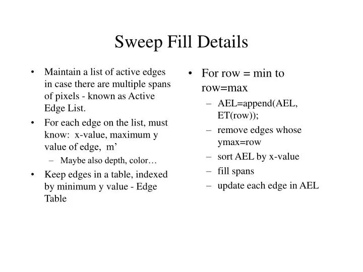
1. Maintain a list of active edges in case there are multiple spans of pixels - known as Active Edge List. For each edge on the list, must know: x-value, maximum y value of edge, m’ Maybe also depth, color… Keep edges in a table, indexed by minimum y value - Edge Table For row = min to row=max AEL=append(AEL, ET(row)); remove edges whose ymax=row sort AEL by x-value fill spans update each edge in AEL Sweep Fill Details

2. Edge Table: A list per row 6 Row: 6 5 5 4 4 4 0 6 3 3 2 2 1 1 2 0 4 6 0 6 1 2 3 4 5 6 6 0 6 ymax xmin 1/m

3. Active Edge List just before filling each row: 6 Row: 6 5 5 4 0 6 6 0 6 4 4 4 0 6 6 0 6 3 3 2 0 4 6 0 6 2 2 2 0 4 6 0 6 1 1 2 0 4 6 0 6 1 2 3 4 5 6 6 0 6 ymax x 1/m

4. Edge Table: Row: 6 6 5 5 4 4 3 3 2 2 1 2 1 5 6 -1 5 1 6 0 6 1 2 3 4 5 6 ymax xmin 1/m

5. Active Edge List just before filling each row: 6 Row: 6 5 5 4 4 3 -1 5 5 1 5 3 3 4 1 5 4 -1 5 2 2 3 1 5 5 -1 5 1 1 2 1 5 6 -1 5 1 2 3 4 5 6 6 0 6 ymax x 1/m

6. Comments • Sort is quite fast, because AEL is usually almost in order • OpenGL limits to convex polygons, meaning two and only two elements in AEL at any time, and no sorting • Can generate memory addresses (for pixel writes) efficiently • Does not require floating point - next slide

7. Dodging Floating Point • For edge, m=x/y, which is a rational number • View x as xi+xn/y, with xn<y. Store xi and xn • Then x->x+m’ is given by: • xn=xn+x • if (xn>=y) { xi=xi+1; xn=xn- y } • Advantages: • no floating point • can tell if x is an integer or not, and get floor(x) and ceiling(x) easily, for the span endpoints • Watt Sect 6.4.1 gives a confusing version

8. Anti-Aliasing • Recall: We can’t sample and then accurately reconstruct an image that is not band-limited • Infinite Nyquist frequency • Attempting to sample sharp edges gives “jaggies”, or stair-step lines • Solution: Band-limit by filtering (pre-filtering) • What sort of filter will give a band-limited result? • But when doing computer rendering, we don’t have the original continuous function

9. Pre-Filtered Primitives • We can simulate filtering by rendering “thick” primitives, with , and compositing • Expensive, and requires the ability to do compositing • Hardware method: Keep sub-pixel masks tracking coverage Filter =1/6 1/6 =2/3 2/3 over =1/6 =1/6 =2/3 1/6 Ideal =1/6 Pre-Filtered and composited

10. Post-Filtering (Supersampling) • Sample at a higher resolution than required for display, and filter image down • Two basic approaches: • Generate extra samples and filter the result (traditional super-sampling) • Generate multiple (say 4) images, each with the image plane slightly offset. Then average the images • Requires general perspective transformations • Can be done in OpenGL using the accumulation buffer • Issues of which samples to take, and how to average them

11. Where We Stand • At this point we know how to: • Convert points from local to window coordinates • Clip polygons and lines to the view volume • Determine which pixels are covered by any given line or polygon • Anti-alias • Next thing: • Determine which polygon is in front

12. Visibility • Given a set of polygons, which is visible at each pixel? (in front, etc.). Also called hidden surface removal • Very large number of different algorithms known. Two main classes: • Object precision: computations that decompose polygons in world to solve • Image precision: computations at the pixel level • All the spaces in the viewing pipeline maintain depth, so we can work in any space • World, View and Window space are all used

13. Visibility Issues • Efficiency - why render pixels many times? • Accuracy - answer should be right, and behave well when the viewpoint moves • Must have technology that handles large, complex rendering databases • In many complex worlds, few things are visible • How much of the real world can you see at any moment? • Complexity - object precision visibility may generate many small pieces of polygon

14. Algorithm: Choose an order for the polygons based on some choice (e.g. depth to a point on the polygon) Render the polygons in that order, deepest one first This renders nearer polygons over further Difficulty: works for some important geometries (2.5D - e.g. VLSI) doesn’t work in this form for most geometries - need at least better ways of determining ordering Painters Algorithm (Image Precision) Fails zs Which point for choosing ordering? xs

15. The Z-buffer (1) (Image Precision)(Watt 6.6.1) • For each pixel on screen, have at least two buffers • Color buffer stores the current color of each pixel • The thing to ultimately display • Z-Buffer stores at each pixel the depth of the nearest thing seen so far • Also called the depth buffer • Initialize this buffer to a value corresponding to the furthest point (z=1.0 for screen and window space) • As a polygon is filled in, compute the depth value of each pixel that is to be filled • if depth < z-buffer depth, fill in pixel color and new depth • else disregard

16. The Z-buffer (2) (Watt 6.6.9) • Advantages: • Simple and now ubiquitous in hardware • A z-buffer is essentially what makes a graphics card “3D” • Computing the required depth values is easy • Disadvantages: • Over-renders - worthless for very large collections of polygons • Depth quantization errors can be annoying • Can’t easily do transparency or filtering for anti-aliasing (Requires keeping information about partially covered polygons)

17. 3rd: To know what to do now Z-Buffer and Transparency • Must render in back to front order • Otherwise, would have to store first opaque polygon behind transparent one Front Partially transparent 1st or 2nd 3rd Opaque 2nd Opaque 1st 1st or 2nd Recall this color and depth

18. OpenGL Depth Buffer • OpenGL defines a depth buffer as its visibility algorithm • The enable depth testing: glEnable(GL_DEPTH_TEST) • To clear the depth buffer: glClear(GL_DEPTH_BUFFER_BIT) • To clear color and depth: glClear(GL_COLOR_BUFFER_BIT|GL_DEPTH_BUFFER_BIT) • The number of bits used for the depth values can be specified (windowing system dependent, and hardware may impose limits based on available memory) • The comparison function can be specified: glDepthFunc(…)

19. The A-buffer (Image Precision)(Watt 14.6) • Handles transparent surfaces and filter anti-aliasing • At each pixel, maintain a pointer to a list of polygons sorted by depth, and a sub-pixel coverage mask for each polygon • Matrix of bits saying which parts of the pixel are covered • Algorithm: When drawing a pixel: • if polygon is opaque and covers pixel, insert into list, removing all polygons farther away • if polygon is transparent or only partially covers pixel, insert into list, but don’t remove farther polygons

20. The A-buffer (2) • Algorithm: Rendering pass • At each pixel, traverse buffer using polygon colors and coverage masks to composite: • Advantage: • Can do more than Z-buffer • Coverage mask idea can be used in other visibility algorithms • Disadvantages: • Not in hardware, and slow in software • Still at heart a z-buffer: Over-rendering and depth quantization problems over =

21. Scan Line Algorithm (Image Precision)(Watt 6.6.5-6.6.7) • Assume polygons do not intersect one another • Except maybe at edges or vertices • Observation: across any given scan line, the visible polygon can change only at an edge • Algorithm: • fill all polygons simultaneously • at each scan line, have all edges that cross scan line in AEL • keep record of current depth at current pixel - use to decide which is in front in filling span

22. Scan Line Algorithm (2) zs zs xs xs Spans zs Where polygons overlap, draw front polygon xs

23. Scan Line Algorithm (3) • Advantages: • Simple • Potentially fewer quantization errors (more bits available for depth) • Don’t over-render (each pixel only drawn once) • Filter anti-aliasing can be made to work (have information about all polygons at each pixel) • Disadvantages: • Invisible polygons clog AEL, ET • Non-intersection criteria may be hard to meet