Download
1 / 39
390 likes | 489 Views
CS505: Intermediate Topics in Database Systems. Jinze Liu. SELECT title, SID FROM Enroll, Course WHERE Enroll.CID = Course.CID;. SQL query. < Query >. Parser. < SFW >. Parse tree. < select-list >. < where-cond >. < from-list >. …. …. Validator. < table >. < table >.

E N D
SELECT title, SIDFROM Enroll, CourseWHERE Enroll.CID = Course.CID; SQL query <Query> Parser <SFW> Parse tree <select-list> <where-cond> <from-list> … … Validator <table> <table> ¼title, SID ¾Enroll.CID = Course.CID Logical plan Enroll Course £ Optimizer PROJECT (title, SID) Enroll Course Physical plan MERGE-JOIN (CID) Executor SORT (CID) SCAN (Course) SCAN (Enroll) Result A query’s trip through the DBMS
Parsing and validation • Parser: SQL ! parse tree • Good old lex & yacc • Detect and reject syntax errors • Validator: parse tree ! logical plan • Detect and reject semantic errors • Nonexistent tables/views/columns? • Insufficient access privileges? • Type mismatches? • Examples: AVG(name), name + GPA, Student UNION Enroll • Also • Expand * • Expand view definitions • Information required for semantic checking is found in system catalog (contains all schema information)
¼title ¾Student.name=“Bart” ÆStudent.SID = Enroll.SIDÆEnroll.CID = Course.CID £ £ Course Student Enroll ¼title An equivalent plan: !Enroll.CID = Course.CID Course !Student.SID = Enroll.SID Enroll ¾name = “Bart” Student Logical plan • Nodes are logical operators (often relational algebra operators) • There are many equivalent logical plans
Physical (execution) plan • A complex query may involve multiple tables and various query processing algorithms • E.g., table scan, index nested-loop join, sort-merge join, hash-based duplicate elimination… • A physical plan for a query tells the DBMS query processor how to execute the query • A tree of physical plan operators • Each operator implements a query processing algorithm • Each operator accepts a number of input tables/streams and produces a single output table/stream
Physical plan execution • How are intermediate results passed from child operators to parent operators? • Temporary files • Compute the tree bottom-up • Children write intermediate results to temporary files • Parents read temporary files • Iterators • Do not materialize intermediate results • Children pipeline their results to parents
Iterator interface • Every physical operator maintains its own execution state and implements the following methods: • open(): Initialize state and get ready for processing • getNext(): Return the next tuple in the result (or a null pointer if there are no more tuples); adjust state to allow subsequent tuples to be obtained • close(): Clean up
An iterator for table scan • State: a block of memory for buffering input R; a pointer to a tuple within the block • open(): allocate a block of memory • getNext() • If no block of R has been read yet, read the first block from the disk and return the first tuple in the block • Or the null pointer if R is empty • If there is no more tuple left in the current block, read the next block of R from the disk and return the first tuple in the block • Or the null pointer if there are no more blocks in R • Otherwise, return the next tuple in the memory block • close(): deallocate the block of memory
An iterator for nested-loop join NESTED-LOOP-JOIN R: An iterator for the left subtree S: An iterator for the right subtree • open() R.open(); S.open(); r = R.getNext(); • getNext() do {s = S.getNext();if (s == null) { S.close(); S.open(); s = S.getNext(); if (s == null) return null; r = R.getNext(); if (r == null) return null;} } until (r joins with s); return rs; • close() R.close(); S.close(); R S Is this tuple-based or block-based nested-loop join?
An iterator for 2-pass merge sort • open() • Allocate a number of memory blocks for sorting • Call open() on child iterator • getNext() • If called for the first time • Call getNext() on child to fill all blocks, sort the tuples, and output a run • Repeat until getNext() on child returns null • Read one block from each run into memory, and initialize pointers to point to the beginning tuple of each block • Return the smallest tuple and advance the corresponding pointer; if a block is exhausted bring in the next block in the same run • close() • Call close() on child • Deallocate sorting memory and delete temporary runs
Blocking vs. non-blocking iterators • A blocking iterator must call getNext() exhaustively (or nearly exhaustively) on its children before returning its first output tuple • Examples: sort, aggregation • A non-blocking iterator expects to make only a few getNext() calls on its children before returning its first (or next) output tuple • Examples: filter, merge join with sorted inputs
Execution of an iterator tree • Call root.open() • Call root.getNext() repeatedly until it returns null • Call root.close() • Requests go down the tree • Intermediate result tuples go up the tree • No intermediate files are needed • But maybe useful if an iterator is opened many times • Example: complex inner iterator tree in a nested-loop join; “cache” its result in an intermediate file
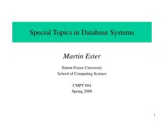
PROJECT (title) PROJECT (title) INDEX-NESTED-LOOP-JOIN (CID) MERGE-JOIN (CID) Index on Course(CID) SCAN (Course) SORT (CID) INDEX-NESTED-LOOP-JOIN (SID) MERGE-JOIN (SID) Index on Enroll(SID) SORT (SID) FILTER (name = “Bart”) INDEX-SCAN (name = “Bart”) SCAN (Enroll) Index on Student(name) SCAN (Student) Examples of physical plans SELECT Course.titleFROM Student, Enroll, CourseWHERE Student.name = ‘Bart’AND Student.SID = Enroll.SID AND Enroll.CID = Course.CID; • Many physical plans for a single query • Equivalent results, but different costs and assumptions! • DBMS query optimizer picks the “best” possible physical plan
Any of these will do 1 second 1 minute 1 hour Query optimization • One logical plan ! “best” physical plan • Questions • How to enumerate possible plans • How to estimate costs • How to pick the “best” one • Often the goal is not getting the optimum plan, but instead avoiding the horrible ones
! ! ! … = = = ! ! ! T T S R S S R R T Plan enumeration in relational algebra • Apply relational algebra equivalences • Join reordering: £ and ! are associative and commutative (except column ordering, but that is unimportant)
More relational algebra equivalences • Convert ¾p-£ to/from !p: ¾p(R£S) = R!pS • Merge/split ¾’s: ¾p1(¾p2R) = ¾p1 Æp2R • Merge/split ¼’s: ¼L1(¼L2R) = ¼L1R, where L1 µL2 • Push down/pull up ¾:¾pÆprÆps (R!p’S) = (¾prR) !pÆp’ (¾psS), where • pr is a predicate involving only R columns • ps is a predicate involving only S columns • p and p’ are predicates involving both R and S columns • Push down ¼: ¼L (¾pR) = ¼L (¾p (¼L L’R)), where • L’ is the set of columns referenced by p that are not in L • Many more (seemingly trivial) equivalences… • Can be systematically used to transform a plan to new ones
¼title ¾Student.name=“Bart” ÆStudent.SID = Enroll.SIDÆEnroll.CID = Course.CID £ £ Course ¼title Student Enroll Convert ¾p-£ to !p Push down ¾ ¾Enroll.CID = Course.CID ¼title £ !Enroll.CID = Course.CID Course ¾Student.SID = Enroll.SID Course £ !Student.SID = Enroll.SID Enroll ¾Student.name = “Bart” Enroll ¾name = “Bart” Student Student Relational query rewrite example
Heuristics-based query optimization • Start with a logical plan • Push selections/projections down as much as possible • Why? Reduce the size of intermediate results • Why not? May be expensive; maybe joins filter better • Join smaller relations first, and avoid cross product • Why? Reduce the size of intermediate results • Why not? Size depends on join selectivity too • Convert the transformed logical plan to a physical plan (by choosing appropriate physical operators)
SQL query rewrite • More complicated—subqueries and views divide a query into nested “blocks” • Processing each block separately forces particular join methods and join order • Even if the plan is optimal for each block, it may not be optimal for the entire query • Unnest query: convert subqueries/views to joins • We can just deal with select-project-join queries • Where the clean rules of relational algebra apply
SQL query rewrite example • SELECT nameFROM StudentWHERE SID = ANY (SELECT SID FROM Enroll); • SELECT nameFROM Student, EnrollWHERE Student.SID = Enroll.SID; • Wrong—consider two Bart’s, each taking two classes • SELECT nameFROM (SELECT DISTINCT Student.SID, name FROM Student, Enroll WHERE Student.SID = Enroll.SID); • Right—assuming Student.SID is a key
Dealing with correlated subqueries • SELECT CID FROM CourseWHERE title LIKE ’CPS%’AND min_enroll > (SELECT COUNT(*) FROM Enroll WHERE Enroll.CID = Course.CID); • SELECT CIDFROM Course, (SELECT CID, COUNT(*) AS cnt FROM Enroll GROUP BY CID) tWHERE t.CID = Course.CID AND min_enroll > t.cntAND title LIKE ’CPS%’; • New subquery is inefficient (computes enrollment for all courses) • Suppose a CPS class is empty?
“Magic” decorrelation • SELECT CID FROM CourseWHERE title LIKE ’CPS%’AND min_enroll > (SELECT COUNT(*) FROM Enroll WHERE Enroll.CID = Course.CID); • CREATE VIEW Supp_Course ASSELECT * FROM Course WHERE title LIKE ’CPS%’; CREATE VIEW Magic ASSELECT DISTINCT CID FROM Supp_Course; CREATE VIEW DS AS(SELECT Enroll.CID, COUNT(*) AS cnt FROM Magic, Enroll WHERE Magic.CID = Enroll.CID GROUP BY Enroll.CID) UNION(SELECT Magic.CID, 0 AS cnt FROM Magic WHERE Magic.CID NOT IN (SELECT CID FROM Enroll); SELECT Supp_Course.CID FROM Supp_Course, DSWHERE Supp_Course.CID = DS.CIDAND min_enroll > DS.cnt; Process the outer querywithout the subquery Collect bindings Evaluate the subquerywith bindings Finally, refinethe outer query
Heuristics- vs. cost-based optimization • Heuristics-based optimization • Apply heuristics to rewrite plans into cheaper ones • Cost-based optimization • Rewrite logical plan to combine “blocks” as much as possible • Optimize query block by block • Enumerate logical plans (already covered) • Estimate the cost of plans • Pick a plan with acceptable cost • Focus: select-project-join blocks
Input to SORT(CID): PROJECT (title) MERGE-JOIN (CID) SCAN (Course) SORT (CID) MERGE-JOIN (SID) SORT (SID) FILTER (name = “Bart”) SCAN (Enroll) SCAN (Student) Cost estimation Physical plan example: • We have: cost estimation for each operator • Example: SORT(CID) takes 2 £B(input) • But what is B(input)? • We need: size of intermediate results
Selections with equality predicates • Q: ¾A = vR • Suppose the following information is available • Size of R: |R| • Number of distinct A values in R: |¼AR| • Assumptions • Values of A are uniformly distributed in R • Values of v in Q are uniformly distributed over all R.A values • |Q| ¼ |R| ⁄ |¼AR| • Selectivity factor of (A = v) is 1 ⁄ |¼AR|
Conjunctive predicates • Q: ¾A = u and B = vR • Additional assumptions • (A = u) and (B = v) are independent • Counterexample: major and advisor • No “over”-selection • Counterexample: A is the key • |Q| ¼ |R| ⁄ (|¼AR| · |¼BR|) • Reduce total size by all selectivity factors
Negated and disjunctive predicates • Q: ¾A¹vR • |Q| ¼ |R| · (1 – 1 ⁄ |¼AR|) • Selectivity factor of :p is (1 – selectivity factor of p) • Q: ¾A = u or B = vR • |Q| ¼ |R| · (1 ⁄ |¼AR| + 1 ⁄ |¼BR|)? • No! Tuples satisfying (A = u) and (B = v) are counted twice • |Q| ¼ |R| · (1 – (1 – 1 ⁄ |¼AR|) · (1 – 1 ⁄ |¼BR|)) • Intuition: (A = u) or (B = v) is equivalent to: ( : (A = u) AND : (B = v))
Range predicates • Q: ¾A > vR • Not enough information! • Just pick, say, |Q| ¼ |R| · 1 ⁄ 3 • With more information • Largest R.A value: high(R.A) • Smallest R.A value: low(R.A) • |Q| ¼ |R| · (high(R.A) – v) ⁄ (high(R.A) – low(R.A)) • In practice: sometimes the second highest and lowest are used instead • The highest and the lowest are often used by inexperienced database designer to represent invalid values!
Two-way equi-join • Q: R(A, B) !S(A, C) • Assumption: containment of value sets • Every tuple in the “smaller” relation (one with fewer distinct values for the join attribute) joins with some tuple in the other relation • That is, if |¼AR| · |¼AS| then ¼ARµ¼AS • Certainly not true in general • But holds in the common case of foreign key joins • |Q| ¼ |R| ¢ |S| ⁄ max(|¼AR|, |¼AS|) • Selectivity factor of R.A = S.A is1 ⁄ max(|¼AR|, |¼AS|)
Multiway equi-join • Q: R(A, B) !S(B, C) !T(C, D) • What is the number of distinct C values in the join of R and S? • Assumption: preservation of value sets • A non-join attribute does not lose values from its set of possible values • That is, if A is in R but not S, then ¼A (R!S) = ¼AR • Certainly not true in general • But holds in the common case of foreign key joins (for value sets from the referencing table)
Multiway equi-join (cont’d) • Q: R(A, B) !S(B, C) !T(C, D) • Start with the product of relation sizes • |R| ¢ |S| ¢ |T| • Reduce the total size by the selectivity factor of each join predicate • R.B = S.B: 1 ⁄ max(|¼BR|, |¼BS|) • S.C = T.C: 1 ⁄ max(|¼CS|, |¼CT|) • |Q| ¼ (|R| ¢ |S| ¢ |T|) ⁄(max(|¼BR|, |¼BS|) ¢ max(|¼CS|, |¼CT|))
Cost estimation: summary • Using similar ideas, we can estimate the size of projection, duplicate elimination, union, difference, aggregation (with grouping) • Lots of assumptions and very rough estimation • Accurate estimate is not needed • Maybe okay if we overestimate or underestimate consistently • May lead to very nasty optimizer “hints” SELECT * FROM Student WHERE GPA > 3.9; SELECT * FROM Student WHERE GPA > 3.9 AND GPA > 3.9; • Not covered: better estimation using histograms
! ! ! ! R2 R1 R3 R4 R5 Search for the best plan • Huge search space • “Bushy” plan example: • Just considering different join orders, there are (2n – 2)! / (n – 1) bushy plans for R1!L!Rn • 30240 for n = 6 • And there are more if we consider: • Multiway joins • Different join methods • Placement of selection and projection operators
! ! R5 ! R4 ! R3 R2 R1 Left-deep plans • Heuristic: consider only “left-deep” plans, in which only the left child can be a join • Tend to be better than plans of other shapes, because many join algorithms scan inner (right) relation multiple times—you will not want it to be a complex subtree • How many left-deep plans are there for R1!L!Rn? • Significantly fewer, but still lots— n! (720 for n = 6)
! Minimize expected size Sk A greedy algorithm • S1, …, Sn • Say selections have been pushed down; i.e., Si = ¾p Ri • Start with the pair Si, Sj with the smallest estimated size for Si!Sj • Repeat until no relation is left:Pick Sk from the remaining relations such that the join of Sk and the current result yields an intermediate result of the smallest size Pick most efficient join method Remainingrelationsto be joined …, Sk,Sl,Sm, … Current subplan
A dynamic programming approach • Generate optimal plans bottom-up • Pass 1: Find the best single-table plans (for each table) • Pass 2: Find the best two-table plans (for each pair of tables) by combining best single-table plans • … • Pass k: Find the best k-table plans (for each combination of k tables) by combining two smaller best plans found in previous passes • … • Rationale: Any subplan of an optimal plan must also be optimal (otherwise, just replace the subplan to get a better overall plan) • Well, not quite…
The need for “interesting order” • Example: R(A, B) !S(A, C) !T(A, D) • Best plan for R!S: hash join (beats sort-merge join) • Best overall plan: sort-merge join R and S, and then sort-merge join with T • Subplan of the optimal plan is not optimal! • Why? • The result of the sort-merge join of R and S is sorted on A • This is an interesting order that can be exploited by later processing (e.g., join, duplicate elimination, GROUPBY, ORDERBY, etc.)!
Dealing with interesting orders • When picking the best plan • Comparing their costs is not enough • Plans are not totally ordered by cost anymore • Comparing interesting orders is also needed • Plans are now partially ordered • Plan X is better than plan Y if • Cost of X is lower than Y • Interesting orders produced by X subsume those produced by Y • Need to keep a set of optimal plans for joining every combination of k tables • At most one for each interesting order
Summary • Relational algebra equivalence • SQL rewrite tricks • Heuristics-based optimization • Cost-based optimization • Need statistics to estimate sizes of intermediate results • Greedy approach • Dynamic programming approach