Download
1 / 1
10 likes | 100 Views
+. Characterizing surface textures on the West Antarctic Ice Sheet. Benjamin Smith Funded by the 2002-05 Earth Systems Science Fellowship and NASA grant NAG5-9906. ben@ess.washington.edu. Transfer coefficient. Glacier surface slope. Ratio of sliding rate to deformation rate.

E N D
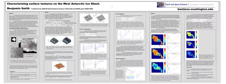
+ Characterizing surface textures on the West Antarctic Ice Sheet. Benjamin Smith Funded by the 2002-05 Earth Systems Science Fellowship and NASA grant NAG5-9906 ben@ess.washington.edu Transfer coefficient Glacier surface slope Ratio of sliding rate to deformation rate Fourier transform of surface log(ratio of near-surface ice viscosity to near-bed ice viscosity) Fourier transform of bed Figure 7: Survey statistics as a function of Co and h. At left, the amplitude Ao as a function of the sliding parameter Co for three different stratification parameters. At right, the solid line shows b1, the short-wavelength spectral exponent, while the dotted line shows b2, the long-wavelength spectral exponent.. Figure 2: transfer amplitudes as a function of strike angle and wavelength of Fourier components. At left, typical conditions for slow-moving inland ice, at right, typical ice-stream conditions. Figure 3: Bed generated using isotropic red noise model with g=-1.5. Models with g>-1.5 have a rougher appearance because they have more spectral power at small wavelength Figure 6: Spectrum shape as a function of wavelength and stratification parameter. At left, spectra for slow sliding, at right, spectra for fast sliding. The slope of the curve at short wavelength becomes steeper, and the transfer at all wavelengths becomes smaller as h increases. Note that the total range of amplitudes is much larger for the slow-sliding case. Figure 5: Spectrum shape as a function of wavelength and surface slope. At left, less stratified conditions with h=4, at right, more stratified conditions with h=8. In the stratified case, there is strong suppression of transfer at short wavelength; in both cases, the shape of the curve as a function of wavelength is consistent, although the amplitude of the transfer increases strongly with slope. Ice flow direction Figure 9. Survey statistics for West Antarctica. At left, model parameters from equation 5. Top left, non-dimensional roughness Ao, defined as the model amplitude at l=6h divided by h. Middle, short-wavelength spectral slope, bottom, long-wavelength spectral slope. At right, example spectra as a function of non-dimensional wavelength l/h. From top to bottom, spectra are for an inter-stream ridge, an ice stream, slow-flowing inland ice, and the ice shelf. Gray lines indicate ice stream margins. Figure 4: Surfaces predicted for the bed in figure 3 and the transfer coefficients in figure 2. The model at left (inland ice: slow sliding, highly stratified) has much less amplitude at short wavelength than the model at right (ice stream, fast sliding, less stratification) Theory I have adapted a theory developed a theory (Gudmundsson, 2003) that predicts ice sheet surface topography for given bed topography. Gudmundsson’s theory approximates an ice sheet as a parallel-sided slab of ice with depth-varying Newtonian viscosity that slides over its bed at a specified rate. The theory gives transfer coefficients that relate the two-dimensional Fourier spectrum of the surface, S(k), to that of the bed, B(k): (1) The transfer coefficients Tsb are defined as a function of two dimensional wave-number k, and of a set of three numbers that define the datum condition of the glacier: a, the surface slope, C0, the ratio of sliding to ice deformation, and X, a parameter that lets the bed-to-surface viscosity variation match that predicted for true nonlinear ice rheology. In general, increasing Co increases the transfer amplitude, especially at small wavelengths. Increasing X stiffens the ice near the surface, leading to less transfer, especially at small wavelengths. Increasing a leads to stronger transfer at all wavelengths (Figure 2). In most parts of Antarctica, the bed topography is not sufficiently well known to be expressed as B(k). Lacking this data, we assume that the bed follows an isotropic red-noise power-law model: (2) Here Bo is a roughness parameter, F is a random phase, and g is the power law exponent describing the spectral shape.. Models of this type have been found to match measured geologic surfaces for g2[-1.5, -0.5] (Turcotte, 1996). Figure 3 shows a bed generated for g=-1.5. Combining the transfer theory with this bed topography model yields a model for ice surface topography defined by five parameters and the ice thickness, h: (3) Figure 4 shows examples of synthetic ice sheet surfaces following equation 3. Abstract The subcontinent of West Antarctica lies beneath ice that is one to two kilometers thick. The ice surface, as seen from space, is white, nearly flat, and nearly featureless, except where shearing ice tears crevasses in the snow. It takes accurate measurements of surface slopes to reveal that the surface is covered with lumps and ripples meters high and kilometers wide that appear as the ice flows over hills and valleys on the glacier bed. I present a spectral analysis of these ripples that characterizes how the kilometer-scale texture of the surface varies across the ice sheet. I distinguish surface spectra that reflect fast-flowing ice from spectra that reflect creeping ice that is frozen to its bed, and demonstrate how the spectral characteristics can be explained by mathematical modeling of ice dynamics in combination with an understanding of the statistics of land surfaces. This analysis presents a powerful tool for making educated guesses about the flow regime in parts of Antarctica where it is not as well understood as in West Antarctica. Results Figure 9 shows estimates of the survey statistics for West Antarctica. To calculate these statistics for real data, the true wavelengths are divided by the ice-thickness to form the non-dimensional wavelength l/h and the spectral amplitude is converted to a non-dimensional amplitude A/h (Ice thickness from the BEDMAP compilation of RADAR data). In the ice streams, we see relatively flat spectra in the short-wavelength region, and small surface amplitudes. In the inland part of the ice sheet, the spectral slope is large, as is the surface power, reflecting mountainous bed-topography and slow sliding. Near the flow-divide, the spectral slope decreases, which may reflect a small amount of sliding at the bed. The inter-stream ridges show some of the strongest slopes at long wavelength seen anywhere. The long-wavelength slope probably results from the change in flow-direction at the ridge-crest, which produces a broad kink in the surface profile that has relatively strong spectral expression at long wavelengths. The ice shelf has both very small spectral slopes and small amplitudes. Althouth there is no bed topography present, short-wavelength topography is slow to decay in stratified ice, so most visible texture is a remnant from when the ice here was grounded. Survey Statistics The dotted lines in figure 4 and 5 show an empirical model for surface spectra that seems to fit most simulated spectra well: (5) lo, the cross-over wavelength, is chosen to be 6.3 h, which corresponds roughly to a wave-number ||k2||=1. The power at this wavelength gives a good estimate of the total spectral power, and corresponds to the typical wavelength of topography seen in shaded-relief imagery of Antarctica. The slopes b1 and b2 describe how the power increases with wavelength at short and long wavelength, respectively. These three parameters are here called survey statistics and can compactly summarize the model behavior over a range of parameters (figure 7). Of course the ice thickness is not known everywhere in Antarctica, so it is instructive to explore what can be done to investigate flow properties using only quantities measurable from the surface. Since the wavelength cannot be made non-dimensional, equation (5) cannot be applied exactly. Rather, I apply the less stringent model consisting of two independent log-log lines: (6) I take a typical ice thickness to be 1000 m , so lo¼6000. Fitting equation 6 to data over a range of wavelengths that does not include lo or adjacent wavelengths allows some flexibility to the model in matching data in which lo¹ 6000. In this case, we can evaluate how well equation 6 fits the data by comparing the wavelength for which A1 exp(b1lx)=A2exp(b2lx) with the ice thickness: if the results at left hold up, lx/6¼ h. With equation 6 we can also find an absolute measure of topographic amplitude at l=6 km from the geometric mean of A1 and A2. As figure 9 makes clear, although the transition wavelength is correlated with ice thickness in the slow-sliding part of the ice sheet, the above technique does not recover the ice thickness with any precision. In the fast-sliding part of the ice-sheet, the slopes at long and short wavelength are quite similar, so the location of the intersection point is not well defined and the estimated ice thickness is badly scattered. Introduction: Surface Texture Defined Most generally defined, surface texture is any undulation of the ice sheet surface that is much smaller in horizontal wavelength than the ice sheet. Practically speaking, surface texture includes a broad range of surface undulations that extend in wavelength from about one kilometer to several tens of kilometers. Figure 1 shows texture in the West Antarctic Ice sheet, where texture varies strongly with local flow conditions. The fast-flowing ice streams, where the ice slides over its bed at up to 1km/year, have the strongest texture, followed by the inland ice, where ice moves mostly by deformation, often over mountainous terrain. The inter-stream ridges have very smooth surfaces, as does stagnant Kamb ice stream. Texture in profile data If the two-dimensional Fourier transform of the ice sheet, S2(k), is known, each component S1(l) of the one-dimensional Fourier transform on a profile parallel to unit-vector v will be approximately (4) a path-integral through the point ko=v 2p/l on a path perpendicular to v. This integral can be evaluated numerically at a range of wavelengths to predict the one-dimensional spectrum. Equation 4 allows the prediction of one-dimensional surface spectra as a function of the datum ice flow, the ice thickness, and the profile azimuth relative to the ice-flow direction, as shown in Figures 5 and 6. Figure 7 shows how the model slopes and amplitude vary as the rate of basal sliding increases. The amplitude increases strongly in a nearly log-linear fashion with the sliding parameter, and decreases as the stratification parameter decreases. Long-wavelength slopes do not vary significantly, but short-wavelength slopes vary greatly, increasing with the sliding parameter and with the stratification parameter. In the slow-sliding regime, where h¼8 and C0 ¼0-1 we can expect to see very low surface amplitudes and consistent short-wavelength spectral slopes on the order of 2.5-3. In the fast-sliding regime, the short-wavelength spectral slope depends strongly on Co. Ice streams Slow inland ice Stagnant ice stream Figure 9: Survey statistics for equation 6. At top, dimensional roughness, middle, measured ice thickness from the BEDMAP consortium, bottom, bottom, estimated ice thickness from the intersection of the model-lines in equation 6. Interstream ridges Measuring spectra Obtaining accurate surface spectra from GLAS data can be complicated where the surface spectrum is strongly dominated by long-wavelength components. I use a modified Welch’s method, using a 3-point Butterworth filter to remove regional trends from the spectrum. Interleaving spectral estimates from different profile-lengths gives good spatial resolution of short-wavelength components, and resolution of long-wavelength components (figure 8). These spectral estimates are interpolated to a grid to give maps of the ice-sheet spectral amplitude at multiple resolutions roughly equally spaced in log(l). Figure 1: Surface texture revealed by shading in West Antarctica. Visible imagery from the AVHRR instrument shows subtle slope variations related to ice-sheet surface texture. Texture at short wavelength is strongest in fast-flowing ice, weaker in slow-flowing inland ice, and absent in interstream ridges and stagnant ice streams Conclusions -A model with simplified ice-sheet dynamics, and a very simple model of bed topography can explain the dominant features of ice-sheet surfaces -The main controls on ice-sheet texture are the sliding rate and the degree of ice-sheet stratification - There are measurable contrasts in ice-surface texture between the slow-sliding part of the ice-sheet and the fast-sliding part -The techniques shown here show promise for estimating flow properties and ice-thickness from surface topography measurements alone, but as yet cannot convincingly do either. Figure 8. Derivation of surface spectra from profile data. Above: location map. At left, elevation profile, running from south to north. Below left, estimation of spectral components between 2 and 50 km. At right, composite spectrum for entire line. References Gudmundsson, G.H. 2003. Transfer of basal variability to the glacier surface. J. Geophys Res. 108: 2253. Huang, J., and D. L. Turcotte. 1989. Fractal mapping of digitized images: Application to the topography of Arizona and comparisons with synthetic images. J. Geophys Res94:7491. Lythe. M.B., Vaughan, D.G., BEDMAP, Consortium. 2001 BEDMAP: a new ice thickness and subglacial topographic model of AntarcticaJ. Geophys Res., 106: 11,335 Ferigno, J.G. Mullins, J.L.,Stapleton, J, Chavez, P.S., Velasco M.G., Williams, R.S., Delinski, G.F., and D'Ann Lear. 2001. AVHRR Image map of Antarctica. (USGS I-2560, 2001).