Download
1 / 33
330 likes | 500 Views
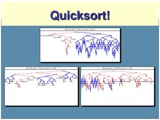
Quicksort!. A practical sorting algorithm. Quicksort Very efficient Tight code Good cache performance Sort in place Easy to implement Used in older version of C++ STL sort(begin, end) Average case performance: O(n log n) Worst case performance: O(n 2 ). Quicksort. Divide & Conquer

E N D
A practical sorting algorithm • Quicksort • Very efficient • Tight code • Good cache performance • Sort in place • Easy to implement • Used in older version of C++ STL sort(begin, end) • Average case performance: O(n log n) • Worst case performance: O(n2)
Quicksort • Divide & Conquer • Divide into two arrays around the last element • Recursively sort each array QUICKSORT Divide around this element
Quicksort • Divide & Conquer • Divide into two arrays around the last element • Recursively sort each array QUICKSORT Dividearound this element
Quicksort • Divide & Conquer • Divide into two arrays around the last element • Recursively sort each array QUICKSORT Exchange
Quicksort • Divide & Conquer • Divide into two arrays around the last element • Recursively sort each array QUICKSORT QUICKSORT
Partitioning the array • PARTITION(A, p, r) • x = A[r] • i = p–1 • for j = p to r-1 • if A[j] <= x • then i++; exchange A[i] and A[j] • exchange A[i+1] and A[r] • return i+1 i j x
Partitioning the array • PARTITION(A, p, r) • x = A[r] • i = p–1 • for j = p to r-1 • if A[j] <= x • then i++; exchange A[i] and A[j] • exchange A[i+1] and A[r] • return i+1 i j x
Partitioning the array • PARTITION(A, p, r) • x = A[r] • i = p–1 • for j = p to r-1 • if A[j] <= x • then i++; exchange A[i] and A[j] • exchange A[i+1] and A[r] • return i+1 i j x
Partitioning the array • PARTITION(A, p, r) • x = A[r] • i = p–1 • for j = p to r-1 • if A[j] <= x • then i++; exchange A[i] and A[j] • exchange A[i+1] and A[r] • return i+1 i j x
Partitioning the array • PARTITION(A, p, r) • x = A[r] • i = p–1 • for j = p to r-1 • if A[j] <= x • then i++; exchange A[i] and A[j] • exchange A[i+1] and A[r] • return i+1 i j x
Putting it together: Quicksort • QUICKSORT(A, p, r) • if p < r • then q = PARTITION(A, p, r) • QUICKSORT(A, p, q-1) • QUICKSORT(A, q+1, r) QUICKSORT QUICKSORT QUICKSORT p q r
Putting it together: Quicksort • PARTITION(A, p, r) • x = A[r]; i = p–1 • for j = p to r-1 • if A[j] <= x • then i++; exchange A[i] and A[j] • exchange A[i+1] and A[r] • return i+1 QUICKSORT(A, p, r) if p < r then q = PARTITION(A, p, r) QUICKSORT(A, p, q-1) QUICKSORT(A, q+1, r) • To sort an array A of length n: • QUICKSORT(A, 1, n)
Running Time • PARTITION(A, p, r) • x = A[r]; i = p–1 • for j = p to r-1 • if A[j] <= x • then i++; exchange A[i] and A[j] • exchange A[i+1] and A[r] • return i+1 QUICKSORT(A, p, r) if p < r then q = PARTITION(A, p, r) QUICKSORT(A, p, q-1) QUICKSORT(A, q+1, r) • PARTITION(A, p, r)Time O(r-p) • Outside loop: • ~5 operations • 0 comparisons • Inside loop: • r-p comparisons • c(r-p) total operations, for some c ~= 5
Running Time • PARTITION(A, p, r) • x = A[r]; i = p–1 • for j = p to r-1 • if A[j] <= x • then i++; exchange A[i] and A[j] • exchange A[i+1] and A[r] • return i+1 QUICKSORT(A, p, r) if p < r then q = PARTITION(A, p, r) QUICKSORT(A, p, q-1) QUICKSORT(A, q+1, r) • QUICKSORT (A, 1, n) • Let T(n) be the worst-case running time, for any n • Then, T(n) ≤ max{1 ≤ q ≤ n-1} ( T(q-1) + T(n-q) + (n) )(why?)
Worst-Case Running Time • Sort A = [n, n-1, n-2, …, 3, 2, 1] • PARTITION(A, 1, n) A = [1, n-1, n-2, …, 3, 2, n] • PARTITION(A, 2, n) A = [1, n-1, n-2, …, 3, 2, n] • PARTITION(A, 2, n-1) A = [1, 2, n-2, …, 3, n-1, n] • PARTITION(A, 3, n-1) A = [1, 2, n-2, …, 3, n-1, n] • PARTITION(A, 3, n-2) A = [1, 2, 3, …, n-2, n-1, n] • PARTITION(A, 4, n-2) • PARTITION(A, 4, n-3) … • PARTITION(A, n/2, n/2+1) Total comparisons: (n-1) + (n-2) + … + 1 = (n2)
Worst-Case Running Time T(n) ≤ max{1 ≤ q ≤ n-1} ( T(q-1) + T(n – q) + (n) ) Substitution Method: • Guess T(n) < cn2 T(n) ≤ max{1 ≤ q ≤ n} ( c(q – 1)2 + c(n – q)2 ) + dn = c×max{1 ≤ q ≤ n} ((q – 1)2 + (n – q)2 ) + dn • This is max for q = 1 (or, q = n) = c(n2 – 2n + 1) + dn = cn2 – c(2n – 1) + dn ≤ cn2, if we pick c such that c(2n – 1) > dn
A randomized version of Quicksort • Pick a random number in the array as a pivot • RANDOMIZED-PARTITION(A, p, r) • i = RANDOM(p, r) • exchange A[r] and A[i] • return PARTITION(A, p, r) • RANDOMIZED-QUICKSORT(A, p, r) • if p < r • then q = RANDOMIZED-PARTITION(A, p, r) • RANDOMIZED-QUICKSORT(A, p, q – 1) • RANDOMIZED-QUICKSORT(A, q + 1, r) • What is the expected running time?
Expected running time of Quicksort • Observe that the running time is a constant times the number of comparison Lemma Let X be the number of comparisons (A[j] <= x) performed by PARTITION. Then, the running time of QUICKSORT is (n+X) Proof There are n calls to PARTITION. Each call does a constant amount of work, plus the for loop. Each iteration of the for loop executes the comparison A[j] <= x. Therefore, running time of PARTITION is a (# comparisons)
A quick review of probability Define a sample space S, which is a set of events S = { A1, A2, …. } Each event A has a probability P(A), such that • P(A) ≥ 0 • P(S) = P(A1) + P(A2) + … = 1 • P(A or B) = P(A) + P(B) More generally, for any subset T = { B1, B2, … } of S, P(T) = P(B1) + P(B2) + …
A quick review of probability • Example: Let S be all sequences of 2 coin tosses S = {HH, HT, TH, TT} • Let each head/tail occur with 50% = 0.5 probability, independent of the other coin flips • Then P(HH) = P(HT) = P(TH) = P(TT) = 0.25 • Let T = “no two tails occurring one after another” = { HH, HT, TH } • Then, P(T) = P(HH) + P(TH) + P(TT) = 0.75
A quick review of probability • A random variable X is a function from S to real numbers X: S R Example: X = “$3 for every heads” X: {HH, HT, TH, TT} R X(HH) = 6; X(HT) = X(TH) = 3; X(TT) = 0
A quick review of probability • Given two random variables X and Y, • The joint probability density function f(x, y) is • f(x, y) = P(X = x and Y = y) • Then, • P(X = x0) = y P(X = x0 and Y = y) • P(Y = yo) = x P(X = x and Y = y0) • The conditional probability • P(X = x | Y = y) = P(X = x and Y = y) / P(Y = y)
A quick review of probability • Two random variables X and Y are independent, if for all values x and y, P(X = x and Y = y) = P(X = x) P(Y = y) Example: X = 1, if first coin toss is heads; 0 otherwise Y = 1, if second coin toss is heads; 0 otherwise Easy to check that X and Y are independent
A quick review of probability • The expected value E(X) of a random variable X, is E(X) = x x P(X = x) • Going back to the coin tosses, estimate E(X) E(X) = 6 P(X = 6) + 3 P(X = 3) + 0 P(X = 0) = 6×0.25 + 3×0.5 + 0×0.25 = 1.5 + 1.5 + 0 = 3
A quick review of probability Linearity of expectation: E(X + Y) = E(X) + E(Y) For any function g(x), E(g(X)) = x g(x) P(X = x) Assume X and Y are independent: E[XY] = xyxyP(X = x and Y = y) = xyP(X = x) P(Y = y) = x P(X = x) yP(Y = y) = E(X) E(Y)
A quick review of probability Define indicator variable I(A), where A is an event 1, if A occurs • I(A) = 0, otherwise Lemma: Given a sample space S, and an event A, E[ I(A) ] = P(A) Proof: E[ I(A) ] = 1×P(A) + 0×P(S – A) = P(A)
Back to Quicksort Lemma Let X be the number of comparisons (A[j] <= x) performed by PARTITION. Then, the running time of QUICKSORT is O(n+X) Define indicator random variables: Xij = I( zi is compared to zj during the course of the algorithm ) Then, the total number of comparisons performed is: X = i=1…n-1j=i+1…n Xij
Expected running time of Quicksort • Running time = X = i=1…n-1 j=i+1…n Xij • Expected running time = E[X] E[X] = E[i=1…n-1j=i+1…n Xij ] = i=1…n-1j=i+1…n E[ Xij ] = i=1…n-1 j=i+1…nP( zi is compared to zj ) • We just need to estimate P( zi is compared to zj )
Expected running time of Quicksort During partition of zi……zj • Once a pivot p is selected • p is compared to all elements except itself • no element < p is ever compared to an element > p smaller than pivot larger than pivot
Expected running time of Quicksort • Denote by Zij = { zi,……,zj } In order to compare zi and zj • First element chosen as pivot within Zij should be zi, or zj P( zi is compared to zj ) = = P( zi or zj is first pivot from Zij ) = P( zi is first pivot from Zij ) + P( zj is first pivot from Zij ) = 1/(j – i +1) + 1/(j – i + 1) = 2/(j – i + 1)
Expected running time of Quicksort Now we are ready to compute E[X]: E[X] = i=1…n-1j=i+1…n 2/(j – i + 1) Let k = j – i E[X] = i=1…n-1j=i+1…n 2/(k + 1) < i=1…n j=1…n2/k = i=1…n(lg n + O(1)) by CLRS A.7 = O(n lg n )
Selection: Find the ith number 2 10 • The ithorder statistics is the ith smallest element 7 13 9 8 11 14 15 6 5 4 3 12 1