Download
1 / 37
390 likes | 589 Views
Crystal Structure Determination and Refinement Using the Bruker AXS SMART APEX System. Charles Campana Bruker Nonius. Flowchart for Method. Adapted from William Clegg “Crystal Structure Determination” Oxford 1998. Crystal Growing Techniques. Slow evaporation Slow cooling

E N D
Crystal Structure Determination and Refinement Using the Bruker AXS SMART APEX System Charles Campana Bruker Nonius
Flowchart for Method Adapted from William Clegg “Crystal Structure Determination” Oxford 1998.
Crystal Growing Techniques • Slow evaporation • Slow cooling • Vapor diffusion • Solvent diffusion • Sublimation http://laue.chem.ncsu.edu/web/GrowXtal.html http://www.as.ysu.edu/~adhunter/YSUSC/Manual/ChapterXIV.pdf
Growing Crystals Kirsten Böttcher and Thomas Pape
Select and Mount the Crystal • Use microscope • Size: ~0.4 (±0.2) mm • Transparent, faces, looks single • Epoxy, caulk, oil, grease to affix • Glass fiber, nylon loop, capillary
Crystallographic Unit Cell Unit Cell Packing Diagram - YLID
7 Crystal Systems - Metric Constraints • Triclinic - none • Monoclinic - = = 90, 90 • Orthorhombic - = = = 90 • Tetragonal - = = = 90, a = b • Cubic - = = = 90, a = b = c • Trigonal - = = 90, = 120, a = b (hexagonal setting) or = = , a = b = c (rhombohedral setting) • Hexagonal - = = 90, = 120, a = b
X-Ray Diffraction Pattern from Single Crystal Rotation Photograph
X-Ray Diffraction X-ray beam 1Å (0.1 nm) ~ (0.2mm)3 crystal ~1013 unit cells, each ~ (100Å)3 Diffraction pattern on CCD or image plate
Bragg’s law We can think of diffraction as reflection at sets of planes running through the crystal. Only at certain angles 2 are the waves diffracted from different planes a whole number of wavelengths apart, i.e., in phase. At other angles, the waves reflected from different planes are out of phase and cancel one another out. n = 2d sin() d
Reflection Indices z These planes must intersect the cell edges rationally, otherwise the diffraction from the different unit cells would interfere destructively. We can index them by the number of times h, k and l that they cut each edge. The same h, k and l values are used to index the X-ray reflections from the planes. y x Planes 3 -1 2 (or -3 1 -2)
Diffraction Patterns Two successive CCD detector images with a crystal rotation of one degree per image For each X-ray reflection (black dot), indices h,k,l can be assigned and an intensity I = F 2 measured
Reciprocal space • The immediate result of the X-ray diffraction experiment is a list of X-ray reflections hkl and their intensities I. • We can arrange the reflections on a 3D-grid based on their h, k and lvalues. The smallest repeat unit of this reciprocal lattice is known as the reciprocal unit cell; the lengths of the edges of this cell are inversely related to the dimensions of the real-space unit cell. • This concept is known as reciprocal space; it emphasizes the inverse relationship between the diffracted intensities and real space.
The structure factor F and electron density Fhkl = Vxyz exp[+2i(hx+ky+lz)] dV xyz = (1/V) hklFhkl exp[-2i(hx+ky+lz)] F and are inversely related by these Fourier transformations. Note that is real and positive, but F is a complex number: in order to calculate the electron density from the diffracted intensities, I = F2, we need the PHASE ( ) of F. Unfortunately it is almost impossible to measure directly! F(h,k,l) = A + iB
The Crystallographic Phase Problem • In order to calculate an electron density map, we require both the intensities I= F 2 and the phases of the reflections hkl. • The information content of the phases is appreciably greater than that of the intensities. • Unfortunately, it is almost impossible to measure the phases experimentally ! This is known as the crystallographic phase problem and would appear to be insoluble
Real Space Unit Cell (a, b, c, , , ) Electron Density, (x, y, z) Atomic Coordinates – x, y, z Thermal Parameters – Bij or Uij Bond Lengths (A) Bond Angles (º) Crystal Faces Reciprocal Space Unit Cell (a*, b*, c*, *, *, *) Diffraction Pattern Reflections – h,h,l Integrated Intensities – I(h,k,l) Structure Factors – F(h,k,l) Phase – (h,k,l) Real Space and Reciprocal Space
CCD Chip Sizes X8 APEX, SMART APEX, 6000, 6500 4K CCD 62x62 mm Kodak 1K CCD 25x25 mm SMART 1000, 1500 & MSC Mercury SITe 2K CCD 49x49 mm SMART 2000
APEX detector • transmission of fiber-optic taper depends on 1/M2 • APEX with direct 1:1 imaging • 1:1 is 6x more efficient than 2.5:1 • improved optical transmission by almost an order of magnitude • allowing data on yet smaller micro-crystals or very weak diffractors. • original SMART: 17 e/Mo photon; APEX: 170 e/Mo photon
SMART ASTRO setup data collection strategy sample screening data collection SAINTPLUS new project change parameters SAINT: integrate SADABS: scale & empirical absorption correction SHELXTL new project XPREP: space group determination XS: structure solution XL: least squares refinement XCIF: tables, reports project database default settings detector calibration
George M. Sheldrick Professor, Director of Institute and part-time programming technician1960-1966: student at Jesus College and Cambridge University, PhD (1966) with Prof. E.A.V. Ebsworth entitled "NMR Studies of Inorganic Hydrides"1966-1978: University Demonstrator and then Lecturer at Cambridge University; Fellow of Jesus College, CambridgeMeldola Medal (1970), Corday-Morgan Medal (1978)1978-now: Professor of Structural Chemistry at the University of GoettingenRoyal Society of Chemistry Award for Structural Chemistry (1981)Leibniz Prize of the Deutsche Forschungsgemeinschaft (1989)Member of the Akademie der Wissenschaften zu Goettingen (1989)Patterson Prize of the American Crystallographic Association (1993) Author of more than 700 scientific papers and of a program called SHELX Interested in methods of solving and refining crystal structures (both small molecules and proteins) and in structural chemistryemail: gsheldr@shelx.uni-ac.gwdg.defax: +49-551-392582
SHELXTL (Bruker Nonius) XPREP (space group det’m) XS (structure solution) XM XE XL (least-squares refinement) XPRO XWAT XP (plotting) XSHELL (GUI interface) XCIF (tables, reports) SHELX (Public Domain)* None SHELXS SHELXD SHELXE SHELXL SHELXPRO SHELXWAT None None CIFTAB SHELXTL vs. SHELX*http://shelx.uni-ac.gwdg.de/SHELX/index.html