Download
1 / 92
1.04k likes | 1.67k Views
Toward More Realistic Pathfinding. Authored by: Marco Pinter. Path finding. How do people find paths? Local knowledge Go downhill Follow the person in front of you Follow the scent of food Global knowledge Consider all possible paths from start to goal

E N D
Toward More Realistic Pathfinding Authored by: Marco Pinter
Path finding • How do people find paths? • Local knowledge • Go downhill • Follow the person in front of you • Follow the scent of food • Global knowledge • Consider all possible paths from start to goal • Assign a cost to each leg of the path • Find path to goal with smallest cost Continuous Discrete
Algorithms for path finding • Uniformed • You don’t have any insight other than what’s immediately before you • Informed • You have some insight, or heuristics that help you choose where to explore
Path finding data structures • Commonly used data structures • Start: where the search must begin • Goal: where the search must terminate • Fringe: locations in the world that define the boundary of knowledge about the paths from Start to Goal
Uniformed search: Uniform-Cost Search • Always expand the lowest-path-cost node • Don’t evaluate the node until it is “expanded”… not when it is the result of expansion
Uniform-Cost Search • Fringe = [S0] • Expand(S) {A1, B5, C15}
Uniform-Cost Search • Fringe = [A1, B5, C15] • Expand(A) = {G11}
Uniform-Cost Search (review) • Fringe = [B5, G11, C15] • Expand(B) {G10}
Uniform-Cost Search (review) • Fringe = [G10, C15] • Expand(G) Goal
Best-first Search Uniform-cost search explored the node that was the closest • With disregard for how far it was from the goal • because we didn’t know that information What if we knew something about the remaining distance to the goal? • How could we take this into account? • The best node on fringe to explore is one that balances cost to reach and cost to goal
Evaluation function: f(n) • Combine two costs • f(n) = g(n) + h(n) • g(n) = cost to get from start to n • h(n) = cost to get to from n to goal
Heuristics • A function, h(n), that estimates cost of cheapest path from node n to the goal • h(n) = 0 if n == goal node
A* (A-star) Search • Don’t simply minimize the cost to intermediate state on fringe… minimize the cost from start to goal… • f(n) = g(n) + h(n) • g(n) = cost to get to n from start • h(n) = cost to get from n to goal • Select node from fringe that minimizes f(n)
A* is Optimal? • A* can be optimal if h(n) satisfies conditions • h(n) never overestimates cost to reach the goal • it is eternally optimisic • f(n) never overestimates cost of a solution through n
A* is Optimal • We must prove that A* will not return a suboptimal goal or a suboptimal path to a goal • Let G be a suboptimal goal node • f(G) = g(G) + h(G) • h(G) = 0 because G is a goal node • f(G) = g(G) > C* (because G is suboptimal)
A* is Optimal • We must prove that A* will not return a suboptimal goal or a suboptimal path to a goal • Let G be a suboptimal goal node • f(G) = g(G) + h(G) • h(G) = 0 because G is a goal node • f(G) = g(G) > C* (because G is suboptimal) • Let n be a node on the optimal path • because h(n) does not overestimate • f(n) = g(n) + h(n) <= C* • Therefore f(n) <= C* < f(G) • node n will be selected before node G
Contours • Because f(n) is nondecreasing • we can draw contours • If we know C* • We only need to explore contours less than C*
Properties of A* • A* expands all nodes with f(n) < C* • A* expands some (at least one) of the nodes on the C* contour before finding the goal • A* expands no nodes with f(n) > C* • these unexpanded nodes can be pruned
A* is Optimally Efficient No other optimal algorithm is guaranteed to expand fewer nodes than A* • (except perhaps eliminating consideration of ties at f(n) = C*) • Compared to other algorithms using same heuristic
Pros and Cons of A* • A* is optimal and optimally efficient • A* is still slow and bulky (space kills first) • Number of nodes grows exponentially with the length to goal • This is actually a function of heuristic, but they all have errors • A* must search all nodes within this goal contour • Finding suboptimal goals is sometimes only feasible solution
A* for video games • Is very common • It will find a path from start to goal • The world is spatially discretized • Produces zigzag effect between cells • Does not produce smooth turns • Does not check for “illegal moves” or for abrupt turning when a unit has a particular turning radius
Removing the Zigzag Effect Can just associate a cost with each turn, but that does not solve the problem entirely. A better smoothing process is to remove as many waypoints as possible.
Removing the Zigzag Effect checkPoint = starting point of pathcurrentPoint = next point in pathwhile (currentPoint->next != NULL) if Walkable(checkPoint, currentPoint->next) // Make a straight path between those points: temp = currentPoint currentPoint = currentPoint->next delete temp from the path else checkPoint = currentPoint currentPoint = currentPoint->next
Removing the Zigzag Effect Checks path from waypoint to waypoint. If the path traveled intersects a blocked location, the waypoint is not removed. Otherwise, remove the waypoint. Leaves “impossible” sections as is.
Adding Realistic Turns Want to be aware of a unit’s turning radius and choose shortest route to destination, in this case the right turn will lead to the shortest route.
Adding Realistic Turns • Calculate the length of the arc plus the line segment for both left and right turns. Shortest path is the one to use.
Adding Legal Turns Several Postprocess Solutions (cheats) • Ignore blocked tiles – obviously bad • Path recalculations – associate a byte with each tile, each bit denoting the surrounding tiles as legal or illegal; may invalidate legal paths from other directions = bad • Decrease turning radius until it is legal – bad for units with constant turning radius (e.g. truck), good for units such as people • Backing up – make a three point turn – good for units such as trucks, weird for people
Adding Legal Turns Problems • Methods shown previously are basically cheats, except for the second one (path recalculations), which can fail to find valid paths • How can we make sure that paths taken are both legal and do not violate the turning radius?
Directional A* Sometimes the only legal path that does not violate the turning radius constraints is completely different from the path that the standard A* algorithm produces. To get around this, Pinter proposes a modification known as Directional A*.
Directional A* First things first • Add an orientation associated with each node, where the orientation can be any one of the eight compass directions • Each node now represented by three dimensions: [x, y, orientation]
Directional A* • Check the path from a parent to a child node, not just whether or not the child is a blocked tile • Consider the orientation at parent and child nodes as well as the turning radius and size of the unit to see if path hits any blocked tiles • Result: a valid path given the size and turning radius of the unit
Directional A* Directional A* does not go directly from a to c because it sees that an abrupt left turn would cause the unit to hit blocked tiles. Thus, waypoint b is found as the shortest legal path.
Directional A* Problem: adding an end orientation • Four common paths
Directional A* • Can easily compute the four common paths and choose the shortest one • Can add smoothing algorithm presented earlier, with the modification of sampling points along a valid curve between two points rather than just a straight line between two points
Expanding the Search • So far, have been using a Directional-8 search • Some paths will fail under this method • Try searching more than one tile away • Directional-24: search two tiles away, rarely fails to find a valid path • Directional-48: search three tiles away, almost never fails to find a valid path
Modifying the Heuristic • Standard A* measures straight line distance from start to goal • Modify so that it measures the shortest curve and line segment as calculated earlier, considering turn radius • If units can go in reverse, consider adding a cost penalty to encourage units to move in reverse only when necessary
Directional A* Limitations • Very slow, constantly uses tables as a means to optimize it (directional table, heuristic table, hit-check table, etc) • Directional-48 may still possibly (though rarely) fail • The four common paths from origin to destination are not the only ones; there is an infinite number of paths
More Optimizations • Timeslice the search • Only use Directional-24 and -48 if a Directional-8 fails • Divide map into regions and pre-compute whether a tile in one region can reach a tile in another • Use two matrices to calculate intermediate search results, one for slow, timesliced searches and the other for faster searches
Summary • Directional A* finds legal paths and realistic turns • Directional A* is slow • Examples only take into account a 2D space partitioned into a grid, but can be extended to support various partitioning methods in 2D or 3D • Suggest standard A* for most units and Directional A* for various large units
Realistic Human Walking Paths Nicholas L. Johnson School of InformationUniversity of Michigan David C. Brogan Computer Science DepartmentUniversity of Virginia
Motivation for walking characters • Scientific and Entertainment Applications Helbing et al. – Escape Panic Helbing et al. – Trails Phantom Menace
Realistic walking paths • Dynamics matters! • Walking dynamics influence what path is generated • CanI cut the corner to dart down the hallway? • Following a path influences walking dynamics • I must slow down to cut the corner • What a character cando influences what it does
Background • Robotics, Animation, Practitioners • Reactive Control • Reynolds’ steering behaviors • Planning • Bandi and Thalmann A* method • Example-based • Choi, Lee, and Shin motion capture library
What do realistic paths look like? • An empirical question • 36 people performed walking experiments • convenience sample of passersby (unpaid) • Video taped and rotoscoped for path acquisition
Five walking experiments • Carry piece of paper from A to B • Return to A andrepeat 3 times • 7 paths generated
Five walking experiments • No Turn • 7 participants
Five walking experiments • Wide Turn • 7 participants
Five walking experiments • Sharp Turn • 9 participants
Five walking experiments • U Turn • 6 participants
Five walking experiments • S Turn • 7 participants