Download
1 / 35
370 likes | 586 Views
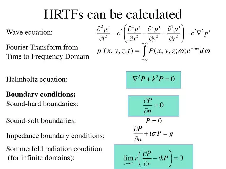
HRTFs can be calculated. Wave equation:. Fourier Transform from Time to Frequency Domain. Helmholtz equation:. Boundary conditions:. Sound-hard boundaries:. Sound-soft boundaries:. Impedance boundary conditions:. Sommerfeld radiation condition (for infinite domains):.

E N D
HRTFs can be calculated Wave equation: Fourier Transform from Time to Frequency Domain Helmholtz equation: Boundary conditions: Sound-hard boundaries: Sound-soft boundaries: Impedance boundary conditions: Sommerfeld radiation condition (for infinite domains):
HRTFs can be computed • Boundary Element Method • Obtain a mesh • Using Green’s function G • Convert equation and b.c.s to an integral equation • Need accurate surface meshes of individuals • Obtain these via computer vision
Current work: Develop Meshes Original Kemar surface points from Dr. Yuvi Kahana,ISVR, Southampton, UK
New quadric metric for simplifying meshes with appearance attributes Hugues Hoppe Microsoft Research Presented by Zhihui Tang
Introduction • Several techniques have been developed for geometrically simplify them. Relatively few techniques account for appearance attributes during simplification. • Metric introduced by Garland and Hecbert is fast and reasonably accurate. They can deal with appearance attribute. • In this paper, developed an improved quadric error metric for simplifying meshes with attributes.
Advantage of the new metric: • intuitively measures error by geometric correspondence • less storage (linear on no. of attributes) • evaluate fast (sparse quadric matrix) • more accurate simplifications(experiments)
What is Triangle Meshes • Vertex 1 x1 y1 z1 Face 1 1 2 3 • Vertex 2 x2 y2 z2 Face 2 1 2 4 • Vertex 3 x3 y3 z3 Face 3 2 4 5 • …… …… • Geometry p R3 • attributesnormals, colors, texture coords, ...
Notation • A triangle mesh M is described by: V , F. • Each vertex v in V has a geometric position pv in R3 and A set of m attribute scalars sv inRm. That is v is in Rm+3.
Previous Quadratic Error Metrics • Minimize sum of squared distances to planes (illustration in 2D)
Simplification of Geometry Qv(v) = Qv1(v)+Qv2(v) Qf(v=(p))=(ntv+d)2=vt(nnt)v+2dntv+d2 =(A,b,c)=((nnt),(dn),d2) Qf is stored using 10 coefficients. Vertex position vmin minimizing Qv(v) is the solution of Av = -b
Simplification of Geometry and Attributes • This approach is to generalize the distances-to-plane metric in R3 to a distance-to- hyperplane in R3+m. • Qf(v)=||v-v’||2 =||p-p’||2+||s-s’||2 • Storage requires (4+m)(5+m)/2 coefficients
New Quadric Error Metric • Qf(v)=||p-p’||2+||s-s’||2
Attribute Discontinuities Example: a crease ,intensities. Modeling such discontinuities needs store multiple sets of attribute values per vertex. Wedges are very useful in this context.
Simplification Enhancements • Memoryless simplification • Volume preservation
Results(I) • Distance between two meshes M1 and M2 is obtained by sampling a collection of points from M1and measuring the distances to the closest points on M2 plus the distances of the same number of points from M2 to M1 • Statistics are reported using L2 norm and L-infinity norm • For meshes with attributes, we also sample attributes at the same points and measure the divisions from the values linearly interpolated at the closest point on the other mesh.