Download
1 / 19
190 likes | 379 Views
Transit detecion on eclipsing binary systems. Hans J. Deeg Instituto de Astrofísica de Canarias. Transit observations in eclipsing binary systems, why and how Transit detection algorithms for EB's Considerations for computing requirements. Why are EB transits of interest to be observed.

E N D
Transit detecion on eclipsing binary systems Hans J. Deeg Instituto de Astrofísica de Canarias • Transit observations in eclipsing binary systems, why and how • Transit detection algorithms for EB's • Considerations for computing requirements
Why are EB transits of interest to be observed The probability to detect planets around EB's with transits is higher: Since the EB plane is aligned with the observer, the planetary one is it likely as well ->higher probability for correct alignement Non-aligned planetary planes would precess around EB rotation axis, and cause periodically transits as well (Schneider, 1994) Detection of circumbinary planets would be a very significant extension to the variety of known planets.
EB Transit lightcurves 1 Time and duration of transits depends on phase of EB during transit.
For longer periodic planets vpl << vEB : trains of several irregularly spaced transits per EB crossing EB transit lightcurves 2: after removal of binary eclipse vpl > vEB vpl > vEB vp l< vEB vpl < vEB P=9d P=9d P=36d P=36d 'Normal' case: planet transits one component complicated shapes: planetary transit during binary eclipse A detection algorithm needs to model these curves by considering all possible periods AND phases of EB at planet crossing
EB Transit detection algorithm (TDA) development Jenkins,Doyle & Cullers 1996: propose a matching filter TDA.The detection statistics C is obtained from a scalar multiplication of the vectors representing model-lc and observed data. Jenkins et al. present this TDA in the context of the transit detection of EBs TEP project (1994-2000; Deeg et al 1998,Doyle et al 2000.) detection statistics is obtained from a comparison of hypotheses transit-present vs transit-absent.
EB transit detecion algorithm, general There is nothing special about them, except for the first step: i) removal of binary eclipses from lightcurve. Use fit obtained from several good observations of eclipses. ii) model signal for Planet(Ei,Pi,{Rpl,ecc}) E: Epoch [E0,..,E0+P] (or phase [0..2]) iii) comparemodel to data -> detection statistical value C(Ei,Pi) within search space [E0,..,E0+P], and [Pmin..Pmax], (Rpl, ecc), repeat steps ii) and iii) for all values of E, P that generate significantly different model signals
EB transit detecion vs single star TD For single star transits: Transits are strictly periodic. Transit shape, duration is invariant against Epoch (slowly varying if eccentric) EB transits: Transits are semi-periodic and shapes/durations depend strongly on planet's epoch Difference of EB algorithms is in the generation of model transits and in finding an efficient way to compare them to the data. -> EB transit detectionis a much larger computational problem than single star TDon the order of the number of epoch steps needed
The TEP project1994-2000, Doyle, Deeg, Schneider, Jenkins et al. Observed CM Dra for 1000hrs (Deeg et al 1998, Doyle et al 2000) TDA: searched data from 1994-98 for P=7-60 days over all phases of CM Dra ~ 2 month computing time with Sun Ultra5 (300MHz) a list of planet candidates was published. Follow-up observations 1999-2001 at predicted transit times did rule out all of them
Algorithm used in TEP Adapted for analysis of ground based data with unknown extinction slope: Compares data to two models: -one with transits (E,P) and extinction fits to all nights (H1) -one without transit, only extinction fit to all nights (H0) Detection stat. C is difference between residuals: C(E,P) = |residH0| – |residH1| This algorithm is NOT specific for eclipsing binaries – but for problematic ground-based data! Doyle et al. 2000
A transit candidate with P ≈ 11d Doyle et al. 2000
tobs P td detc. stat. Planet (E,P) c=1 Model (E,P) c=1/2 Model (E+E,P) , E=td/2 c=1/2 Model (E,P+P) , P=P td/tobs Computational Requirements: TD stepsize Minimum TD step sizes to not miss a transit (Jenkins et al. 1996): If a planet (E,P) is tested by a detection test with (P±P,E) or (P,E±E), its detection statistics is reduced 'signficantly' (to 1/2 in case of correlation).
Computational Requirements 1 Number of epoch and period steps in TDA: tobs: duration of observations td : duration of transit ( fundamental mesh size) P : period of planet in Epoch: E=td/2 -> NE= P / DE = 2 P /td in Period: P=P td/tobs-> NP= (tobs/td) ln(Pmax/Pmin) total: Nstep≈ 2 tobs td-2 (Pmax - Pmin) Ignored here is a weak dependency of td ~ P1/3
Computational Requirements 2 Total Number of operations of TDA: Nop = k Nstep Npts, = k2 tobs td-2 (Pmax - Pmin) Npts where k is a factor depending on the TDA used (k might be < 1), Npts is the number of data pts. For equidistant points: Npts = tobs/tinc and then: Nop = k 2 td-2(Pmax-Pmin) tobs2tinc-1 (1) Examples: (k =1, Pmin=7d, Pmax=60d, td =0.0139d = 20min) TEP: Nop ≈ 2 .1013 (tobs = 1526d, Npts=24 874) COROT: Nop ≈ 1.1 .1012(tobs=150d, Npts=13 500, tinc=16min) Kepler/Eddi: Nop ≈1.0 .1014(tobs=1100d, Npts= 158 000, tinc=10min)
Slicing the lightcurve: saving computing steps Principle: running a TDA on shorter sections of a lightcurve, and co-adding detection statistics from individual sections. If a lightcurve of Npts points is divided into ns sections of Npts,s points, of length tobs,s, the computing requirement Nop,s for each section is: Nop,s = k 2 td-2(Pmax-Pmin) tobs,s Npts,s. The total number of operations is then given by: Nop = ns Nop,s = k 2 td-2(Pmax-Pmin) tobs,s Npts(2) i.e. Nop is reduced by tobs/tobs,s against (1) This scheme was used by TEP project, dividing the observations of tobs=1529d into 5 sections corresponding to the yearly (1994-1998) observing seasons, using tobs = 200d for each of them (mid-march to october). Savings: 1526/200 ≈ 7.6 Only this made the computation feasable with a CPU time of 2 months
Once maxima in C(Ei,Ti) map are found, TDA needs to be rerun with a finer mesh (td,fine ≈ 1/4 td) in small area in E,P around all maximum to find best value of C in (E,P) space. In TEP, this fine-mesh search was performed around the 5000 highest maxima -> final list of planet candidates, subject to follow-up observations Slicing: Adding of detection statistics maps C(E,P) of small region around a candidate with P≈36d, using td = 20min, tobs=200d 1994 (186h) 1995 (185h) 1997 (250h) 1996 (246h) 36,7d P 36,1d JD0+0 JD0+3 E dominant lines are caused by individual features in lightcurve epoch E is an offset {0 ..P} from reference Epoch JD0=2450000 (9 Oct 1995) Bright: high C(E,P) 94-96 94-97 coadded C(E,P) arrays:
Slicing for equidistant data starting from (2) : Nop = k 2 td-2(Pmax-Pmin) tobs,s Npts with Npts = tobs/tincthe total number of computations is: Nop = k 2 td-2(Pmax-Pmin) tobs,stobstinc-1 (3) now, Nop tobs , instead of Nop tobs2 without 'slicing'. Savings from slicing is ns.. Drawbacks: added complexity. Slicing allows running the TDA on shorter sections of data, with the possiblitity to add matrizes C of later data at any time (useful for missions with long tobs)
Analysis of COROT EB data vs TEP -data span only 150 days, not 5 years as in TEP -homogenous noise characteristics in data set -no atmosphere with ‘unkown’ extinction -computers became faster • With O(100) EB's to analyze in COROT fields, no serious computing obstacles are expected. • Selection of best TDA-kernel (matched filter, BLS,..) is TBD and requires lightcurves with realistic noise simulations.
Summary 1. algorithms to analyze EB lightcurves: fundamentally similar to single stars; need to model more complex transits; more 'tricky' to obtain efficient transit detection, as there are fewer invariants in transit lightcurves. 2. Slicing the data into smaller sections improves computational efficiency of TDA, adding complexity. Also, allows efficient adding of additional data. ¿How useful may this method be to single star TD? - TBD 3. COROT EB analysis is not expected to cause serious difficulties. Selection of best TDA is TBD
References Deeg, H.J., et al.1998, A&A 338, 479 Doyle, L.R., et al. 2000, ApJ, 535, 338 Jenkins, J. M.; Doyle, L. R.; Cullers, D. K. 1996, Icarus 119, 244 Schneider, J. 1994, Planet Space Sci. 42, 539