Download
1 / 43
430 likes | 489 Views
Varying Model Parameters And Their Relation To Ensembles. Nick Bassill AOS 900 Wednesday, November 4 th. A Look At The Future …. Ideally, real-time modeling systems will eventually contain these two things: - An ensemble with hundreds (thousands? more?) of members

E N D
Varying Model Parameters And Their Relation To Ensembles Nick Bassill AOS 900 Wednesday, November 4th
A Look At The Future … • Ideally, real-time modeling systems will eventually contain these two things: - An ensemble with hundreds (thousands? more?) of members - A perfect statistical framework for accurately interpreting this vast amount of data • We are arguably closer to realizing the first of these goals • Currently, modeling systems have on the order of 101 of ensemble members
What Is An “Ensemble”? • An ensemble is a collection of different model simulations (“members”) performed for the same area (for example, the Atlantic Ocean) • However, each simulation will have different characteristics, such as: • Different initial conditions • Different dynamical cores • Different grid spacings • Different physics options (i.e. variable parameterizations)
An Ensemble Example – Initial Time From: http://www.nco.ncep.noaa.gov/pmb/nwprod/analysis/
An Ensemble Example – 120 Hours From: http://www.nco.ncep.noaa.gov/pmb/nwprod/analysis/
Now, Starting From The Beginning … • The complexity of numerical models is strongly tied to available computer power • Therefore, models did not really exist before the 1960s • Early models were largely idealized models not designed for day-to-day forecasting, or even for simulating past events • These models often did not incorporate complex, yet important processes such as latent heat release, radiational effects, or boundary layer processes
The Beginning … Continued • These models also used a very coarse resolution (i.e. large grid spacing with few vertical levels) • All of these factors made ensemble creation essentially impossible until much later • However, once sufficient computer power became available
Computational Advances http://en.wikipedia.org/wiki/File:Transistor_Count_and_Moore%27s_Law_-_2008.svg
Data Storage Advances http://en.wikipedia.org/wiki/File:Hard_drive_capacity_over_time.svg
Parameterizations • The AMS Glossary defines a parameterization as “the representation, in a dynamic model, of physical effects in terms of admittedly oversimplified parameters, rather than realistically requiring such effects to be consequences of the dynamics of the system” • Therefore, in many ways parameterizations are inherently unrealistic • However, they are preferable to the alternative of not including important processes *http://amsglossary.allenpress.com/glossary/search?id=parameterization1
Parameterizations Continued • Some common parameterizations are boundary layer parameterizations, cumulus parameterizations, microphysics parameterizations, and shortwave/longwave radiation parameterizations, among many others • For example, a computer could never simulate the motion of every droplet in a cloud, or the latent heat released or absorbed by the formation or dissipation of every cloud droplet • However, given some understanding of the atmosphere, a parameterization can make reasonable guesses for things like droplet fall speed, latent heat release, phase conversions, etc.
Cumulus Parameterizations • Cumulus clouds generally have a scale of roughly 1 km • However, even current real-time high-resolution models only have a grid spacing of about 4 km • This necessitates the need for cumulus parameterizations (CPs) for most models • CPs are one of the more well-known parameterizations, as well as one of the first to be used in sensitivity experiments
From: http://www.mmm.ucar.edu/mm5/documents/MM5_tut_Web_notes/MM5/mm5.htm
Rosenthal (1979) • Rosenthal was the first to vary any sort of model parameter • However, given limited computer power, his model was an idealized hydrostatic, axisymmetric model of a tropical cyclone (TC) with a 20 km horizontal grid spacing • Rosenthal studied the effect of varying his choice of CP on the TC in his simulation
Rosenthal Continued • Rosenthal demonstrated that changing the CP in his model could significantly alter the evolution (size, intensity) of the tropical cyclone he was simulating • Studies like this led to other similar research, with ever-increasing model complexity (and therefore realism) • As time continued, operational models were developed that were non-hydrostatic, and which included much more detailed and improved parameterizations
Baik et al. (1991) • Baik et al. performed a very similar study to that of Rosenthal, in that he varied CPs while using almost the identical model • In this study, Baik et al. also varied individual parameters within each CP, such as evaporation and condensation • They demonstrated that using a CP at this grid-spacing produced a more realistic result than not using one • Similar to Rosenthal, they also found large differences between different CPs
Baik et al. Continued • Changing the CP used, as well as changing the characteristics of latent heat release significantly impact the profile of heating • Heating maxima in the lower troposphere are more conducive to rapid TC strengthening
Puri and Miller (1990) • Puri and Miller used the operational ECMWF model to study the sensitivity of several Australian TCs to choice of CP • They determined that different CPs led to different track and intensity forecasts • Additionally, they found that different CPs created different storm structures, with different heating rates
Lord et al. (1984) • Lord et al. used an axisymmetric, nonhydrostatic model with a 2 km horizontal grid spacing in order to study the effects of varying microphysics parameterizations (MPs) on simulations of hurricanes without the use of a CP • They compared a simulation with only liquid hydrometeors to one where ice was included • Although they both reached similar final intensities, their evolution was quite different
From: http://www.mmm.ucar.edu/mm5/documents/MM5_tut_Web_notes/MM5/mm5-16.gif
Lord et al. Continued • Ice processes produced downdrafts, due to localized cooling directly below the melting layer • These are important for features such as concentric eyewall development
McCumber et al. (1991) • McCumber et al. studied the sensitivity of tropical convection to varying the MP by comparing simulations to radar data • They determined that more complex MPs produced more accurate simulations (i.e. MPs incorporating ice processes did better than those without ice processes) • Furthermore, different MPs produced different heating rates, even ones which included the same numbers of ice processes • This was due primarily to the different fall speeds of the different particles
McCumber et al. • Microphysics are complicated! • Microphysics are highly variable, depending on how many different water types are included, and how they interact
Parameterization Interactions In Numerical Weather Prediction Models From: http://www.mmm.ucar.edu/mm5/documents/MM5_tut_Web_notes/MM5/mm5.htm
Wang and Seaman (1997) • Wang and Seaman compared the effectiveness of different parameterizations andgrid spacings for a variety of events • They examined a number of variables such as light and heavy precipitation (their focus), temperature, sea-level pressure, and winds • One of the key features of their study was the use of sophisticated statistical tools (such as threat scores and bias scores), which is the first such analysis to be performed in a study which varies parameterizations or grid spacings
Wang and Seaman Conclusions • They concluded that different grid spacings and CPs responded differently to different situations • For example, grid spacing did not matter for forecasting light precipitation, but smaller grid spacings improved forecasting of heavy precipitation • Also, some CPs performed best for warm season precipitation, and some performed best for cold season precipitation • “… and the predictive skill of each CPS has a fairly large case-to-case variation in the warm-season events. None of the schemes consistently out performs the others by a wide margin or in all measures of skill.”
Zhu and Zhang (2006) • Zhu and Zhang simulate the evolution of Hurricane Bonnie (1998), while varying the MP variables • They found that while the forecast tracks were similar, the intensities varied considerably • While the simulation without ice processes was the weakest, they discovered that it could artificially be made to be like the others if the latent heat of freezing/melting were artificially added (even though the model didn’t actually include frozen particles)
Zhu and Zhang Continued • The importance of latent heating is made very evident in their experiments
Fovell and Corbosiero (2009) • Fovell and Corbosiero used idealized simulations to determine the effect varying MP parameters have on tropical cyclone motion • They found that the MP without ice processes produced a much more northward track, due to enhanced Beta drift caused by the storm’s large size
Fovell and Corbosiero Continued • The absence of ice allows for a much larger anvil, and therefore a larger storm • However, by manipulating the fall speed of hydrometeors, any MP simulation can effectively by made to reproduce another
Stensrud et al. (2000) • Stensrud et al. compare two different ensembles for short-term MCS forecasting: - one ensemble used the same physics packages, but different initial conditions - one ensemble used the same initial conditions, but different physic packages • Like Wang and Seaman (1997), they use a number of statistical techniques to determine which is “best” • Also like Wang and Seaman (1997), they determined that different situations result in better performances for one ensemble versus another
Stensruds et al. Conclusions • They concluded the physics ensemble is more successful when the large-scale forcing is weak • The initial condition ensemble is more successful for strong large-scale forcing • However, the variance in ensemble members increases 2-6 times faster for the physics ensemble • This makes the physics ensemble more useful from a forecasting perspective, because it will include more potential solutions
Stensrud et al. final suggestion: Combine these two types of ensemble concepts into one to produce a superior result! Here’s a conceptual model:
General Conclusions • Clearly, research using numerical weather prediction models had to wait until computer technology advanced sufficiently • Additionally, the concept of ensembles didn’t really develop until an adequate amount of research had been accomplished such that people realized that changing initial conditions, parameterizations, dynamical cores, etc., produced different forecasts • As shown in these studies (and many others), choice of parameterization can have a profound effect on forecasts
Current/Future Research • Studies such as these reinforce the notion that no one parameterization is “best” for all situations • However, it seems possible to predict in advance which parameterizations will be biased (and in which way) for a given event • This implies that a collection (or ensemble) of parameterizations might be the best approach to forecasting an event or series of events • The current endeavor is to compare the effectiveness of an ensemble comprised of different parameterizations to an ensemble comprised of different initial and boundary conditions
References Baik, J.J., M. DeMaria, and S. Raman, 1991: Tropical Cyclone Simulations with the Betts Convective Adjustment Scheme. Part III: Comparisons with the Kuo Convective Parameterization. Mon. Wea. Rev., 119, 2889–2899. Fovell, R.G., K.L. Corbosiero, and H.C. Kuo, 2009: Cloud Microphysics Impact on Hurricane Track as Revealed in Idealized Experiments. J. Atmos. Sci., 66, 1764–1778. Lord, S.J., H.E. Willoughby, and J.M. Piotrowicz, 1984: Role of a Parameterized Ice-Phase Microphysics in an Axisymmetric, Nonhydrostatic Tropical Cyclone Model. J. Atmos. Sci., 41, 2836–2848. McCumber, M., W.K. Tao, J. Simpson, R. Penc, and S.T. Soong, 1991: Comparison of Ice Phase Microphysical Parameterization Schemes Using Numerical Simulations of Tropical Convection. J. Appl. Meteor., 30, 985–1004. Puri, K., and M. Miller, 1990: Sensitivity of ECMWF Analyses-Forecasts of Tropical Cyclones to Cumulus Parameterization. Mon. Wea. Rev., 118, 1709–1742. Stensrud, D., J. Bao, and T. Wagner, 2000: Using Initial Condition and Model Physics Perturbations in Short-Range Ensemble Simulations of Mesoscale Convective Systems. Mon. Wea. Rev., 128, 2077–2107. Rosenthal, S.L., 1979: The Sensitivity of Simulated Hurricane Development to Cumulus Parameterization Details. Mon. Wea. Rev., 107, 193–197. Wang, W., and N.L. Seaman, 1997: A Comparison Study of Convective Parameterization Schemes in a Mesoscale Model. Mon. Wea. Rev., 125, 252–278. Zhu, T., and D.L. Zhang, 2006: Numerical Simulation of Hurricane Bonnie (1998). Part II: Sensitivity to Varying Cloud Microphysical Processes. J. Atmos. Sci., 63, 109–126.