Download
1 / 11
110 likes | 317 Views
Scenario loop. IS = 1, M Change management variables (X) from one scenario to the next. Iteration loop. IT = 1, N. Next scenario. Scenarios and Sensitivity Analysis.

E N D
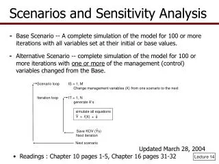
Scenario loop IS = 1, M Change management variables (X) from one scenario to the next Iteration loop IT = 1, N Next scenario Scenarios and Sensitivity Analysis - Base Scenario -- A complete simulation of the model for 100 or more iterations with all variables set at their initial or base values. - Alternative Scenario -- complete simulation of the model for 100 or more iterations with one or more of the management (control) variables changed from the Base. Updated March 28, 2004 • Readings : Chapter 10 pages 1-5, Chapter 16 pages 31-32 Lecture 14
Scenario Analysis - All values in the model are held constant but systematically change one or more control variables • Number of scenarios is determined by anaylst • Random number Seed is held constant • Use =Scenario( ) functions to increment the control variables - Example is to change acres and fixed costs in the model Acre = Scenario (100, 200, 300, 400) FC = Scenario (10, 1000, 5000, 10000) - The control variables make up a scenario table that is incremented by Simetar as model simulates each scenario Lecture 14
Lecture 14 Scenario.XLS Demonstrates Use of 2 Scenarios Lecture 14
Simulating Multiple Scenarios with Different Means Using Simetar Lecture 14
Example of a Scenario Table in Lecture 14 Scenario.XLS • Simetar set for 4 Scenarios • Scenario variables • Acres • Fixed Costs • Mean Yield • Mean Price • KOV is Net Returns • Simetar uses same random numbers for each scenario • Only difference is due to scenario values Lecture 14
Results of the Scenario Analysis Lecture 14
Sensitivity Analysis • Sensitivity analysis seeks to determine how sensitive the KOV is to changes in one particular variable in the model. - For example, does Net Return change a little or a lot when you change variable cost per yield unit in • Simulate the model several times changing the variable in question a given amount and observing the resulting KOV • Each time the model is simulated, it uses the same random numbers so we can compare one run to another, like a scenario analysis Lecture 14
Sensitivity Analysis (continued) Simulation engine expands for sensitivity analysis - Simetar makes sensitivity analysis easy by allowing you to pick a variable to be systematically changed or manipulated • Pick the variable • Type in the percentage changes for the variable to manipulate • Specify the KOVs • Simulate the model • Produce stochastic results for the output variables given the 7 levels for the manipulated variable Lecture 14
Demonstrate Sensitivity Simulation • Use Excel file Scenario.XLS • Change the Variable Costs per Acre as follows • + or – 10% • + or – 5% • + or – 3% • Simulates the model 7 times • The initial value you typed in • Two runs for + and – 10% • Two runs for + and – 5% • Two runs for + and – 3% • Collect the statistics for only the Net Returns KOV • For demonstration purposes collect results for the variable doing the sensitivity test on • Could collect the results for several KOVs Lecture 14
Sensitivity Results Base -10% -5% -3% +3% +5% +10% Base -10% -5% -3% +3% +5% +10% Lecture 14
Sensitivity Results Lecture 14