Download
1 / 14
160 likes | 381 Views
The Job Shop Problem. Chapter 11 Elements of Sequencing and Scheduling by Kenneth R. Baker Byung-Hyun Ha. Outline. Introduction Types of Schedules Disjunctive Programming Schedule Generation Shifting Bottleneck Procedure. Introduction. Job shop model

E N D
The Job Shop Problem Chapter 11 Elements of Sequencing and Schedulingby Kenneth R. Baker Byung-Hyun Ha
Outline • Introduction • Types of Schedules • Disjunctive Programming • Schedule Generation • Shifting Bottleneck Procedure
Introduction • Job shop model • Each job has operations with precedence constraint • Each operation should be done by a specific machine • Representation of a job • (i, j, k) -- operation j of job i requires machine k • Example • 4 jobs with 3 operations and 3 machines Processing time Machine assignment
Introduction • Two views of a feasible schedule • 4 jobs with 3 operations and 3 machines (cont’d) 221 111 431 331 Machine 1 Machine 2 212 412 322 122 Machine 3 313 423 233 133 111 122 133 Job 1 Job 2 212 221 233 Job 3 313 322 331 Job 4 412 423 431
431 331 221 111 412 322 212 122 423 313 233 133 431 331 221 111 412 322 212 122 423 313 233 133 Types of Schedule • Semi-active schedules • Idle time is not helpful for regular measures • Local left-shift • Adjusting start time of operations earlier, without altering the sequence, lest superfluous idle time exists
Types of Schedule • Semi-active schedules (cont’d) • Dominant set w.r.t. regular measures • Number of semi-active schedules -- not more than (n!)m • Network model • Precedence constraints • Disjunctive arcs 2 jobs and 2 machines, 3 jobs and 2 machines Machine assignment 111 122 212 221 1,1 1,2 311 212 2,1 2,2
Types of Schedule • Semi-active schedules (cont’d) • Schedule generation using network model • Resolve disjunctive arcs • Schedule schedulable operation, all of whose predecessors are already scheduled • Resulting schedules are semi-active, some are infeasible • Longest path is makespan 1,1 1,2 1,1 1,2 1,1 1,2 2,1 2,2 2,1 2,2 1,1 1,2 1,1 1,2 2,1 2,2 2,1 2,2 2,1 2,2
431 331 221 111 412 322 212 122 423 313 233 133 111 431 331 221 412 322 212 122 313 423 133 233 Types of Schedule • Active schedules • Global left-shift • Altering sequence and begin some operation earlier, without delaying any other operations • Subset of semi-active schedules and dominant w.r.t. regular measures
111 431 221 331 412 212 122 322 313 423 133 233 111 331 221 431 412 322 212 122 313 423 133 233 Types of Schedule • Nondelay schedules • No machine is kept idle at a time when it could begin processing some operations • No guarantee that nondelay schedules contain an optimum
Types of Schedule • Summary nondelay schedules semi-active schedules active schedules optimum?
Disjunctive Programming • Notation • M -- set of machine • (i, j) -- operation of job j on machine i • pij -- processing time of operation (i, j) • N -- set of all the operations • A NN -- set of precedence constrains of the jobs. • yij -- starting time of operations (i, j) • Objective • min. Cmax • subject to • yij + pij ykj ((i, j), (k, j))A • yij + pij Cmax (i, j)N • yij + pij yilor yil + pil yij (i, j) and (i, l) for i M • yij 0 (i, j)N
Schedule Generation • Algorithm 1 -- Active Schedule Generation 1. Let k = 0 and begin with PS(k) as the null partial schedule. Initially, SO(k) includes all operations with no predecessors. 2. Determine f* = minjSO(k) {fj} and the machine m* on which f* could be realized. 3. For each operation j SO(k) that requires machine m* and for whichsj f*, create a new partial schedule in which operation j is added to PS(k) and started at time sj. 4. For each new partial schedule PS(k + 1) created in Step 3, update the data set as follows: (a) Remove operation j from SO(k). (b) Form SO(k + 1) by adding the direct successor of j to SO(k). (c) Increment k by one. 5. Return to Step 2 for each PS(k + 1) created in Step 3, and continue in this manner until all active schedules have been generated. sj -- the earliest time at which operation j SO(k) could be started sj -- the earliest time at which operation j SO(k) could be finished
Schedule Generation • Using Algorithm 1 • Generating only nondelay schedule • Modifying Step 2 and 3 • Branch and bound • Employing lower bound • Dispatching • Modifying Step 3 and employing priority rules (e.g. SPT, FCFS, MWKR, ...)
Shifting Bottleneck Procedure • Shifting Bottleneck Procedure • Most effective optimization algorithm for job shop problems • Overall procedure • Repeat • Identify the next bottleneck machine • Solving HBT (head-body-tail) problem • Schedule all of the operations of the machine