Download
1 / 25
250 likes | 381 Views
Root Cause Analysis of Failures in Large-Scale Computing Environments. Alex Mirgorodskiy, University of Wisconsin mirg@cs.wisc.edu Naoya Maruyama, Tokyo Institute of Technology naoya.maruyama@is.titech.ac.jp Barton P. Miller, University of Wisconsin bart@cs.wisc.edu http://www.paradyn.org/.

E N D
Root Cause Analysis of Failures in Large-Scale Computing Environments Alex Mirgorodskiy, University of Wisconsin mirg@cs.wisc.edu Naoya Maruyama, Tokyo Institute of Technology naoya.maruyama@is.titech.ac.jp Barton P. Miller, University of Wisconsin bart@cs.wisc.edu http://www.paradyn.org/
Motivation • Systems are complex and non-transparent • Many components, different vendors • Anomalies are common • Intermittent • Environment-specific • Users have little debugging expertise Finding the causes of bugs and performance problems in production systems is hard
Vision Agent Host A Process P Host B network Process R Process Q Autonomous, detailed, low-overhead analysis: • User specifies a perceived problem cause • The agent finds the actual cause
Applications • Diagnostics of E-commerce systems • Trace the path each request takes through a system • Identify unusual paths • Find out why they are different from the norm • Diagnostics of Cluster and Grid systems • Monitor behavior of different nodes in the system • Identify nodes with unusual behavior • Find out why they are different from the norm • Example: found problems in SCore middleware • Diagnostics of Real-time and Interactive systems • Trace words through the phone network • Find out why some words were dropped
Key Components • Data collection: self-propelled instrumentation • Works for a single process • Can cross the user-kernel boundary • Can be deployed on multiple nodes at the same time • Ongoing work: crossing process and host boundaries • Data analysis: use repetitiveness to find anomalies • Repetitive execution of the same high-level action OR • Repetitiveness among identical processes (e.g., Cluster management tools, Parallel codes, Web server farms)
Focus on Control Flow Anomalies • Unusual statements executed • Corner cases are more likely to have bugs • Statements executed in unusual order • Race conditions • Function taking unusually long to complete • Sporadic performance problems • Deadlocks, livelocks
Current Framework P1 • Traces control flow of all processes • Begins at process startup • Stops upon a failure or performance degradation • Identifies anomalies: unusual traces • Problems on a small number of nodes • Both fail-stop and not • Identifies the causes of the anomalies • Function responsible for the problem Trace of P1 P2 P4 P3
Inject instrumenter.so Propagate Analyze: build call graph/CFG with Dyninst Activate a.out 83f0: 83f1: 83f3: 8400: 8405: 8413: 8414: push mov ... call mov pop ret %ebp %esp,%ebp foo %ebp,%esp %ebp bar Patch1 call call jmp instrument(foo) foo 0x8405 jmp patch jmp 8430: 8431: 8433: 8444: 8446: 8449: 844b: 844c: push mov ... call mov xor pop ret %ebp %esp,%ebp *%eax %ebp,%esp %eax,%eax %ebp foo Patch2 call call jmp instrument(%eax) *%eax 0x8446 jmp /dev/instrumenter OS Kernel patch jmp Patch3 sys_call: %eax *%eax push ... call ... iret instrument(%eax) *%eax 0x6d27 call call jmp 6cf5: 6d20: 6d27: 6d49: jmp
Data Collection: Trace Management • The trace is kept in a fixed-size circular buffer • New entries overwrite the oldest entries • Retains the most recent events leading to the problem • The buffer is located in a shared memory segment • Does not disappear if the process crashes ret foo call foo … Process P Tracer
Data Analysis: Find Anomalous Host • Check if the anomaly was fail-stop or not: • One of the traces ends substantially earlier than the others -> Fail-stop • The corresponding host is an anomaly • Traces end at similar times -> Non-fail-stop • Look at differences in behavior across traces P1 P2 Traces P3 P4 Trace end time
Data Analysis: Non-fail-stop Host Find outliers (traces different from the rest): • Define a distance metric between two traces • d(g,h) = measure of similarity of traces g and h • Define a trace suspect score • σ(h) = similarity of h to the common behavior • Report traces with high suspect scores • Most distant from the common behavior
Defining the Distance Metric t(bar) δ(g,h) p(g) p(h) t(foo) • Compute the time profile for each host h: • p(h) = (t1, …, tF) • ti = normalized time spent in function fi on host h • Profiles are less sensitive to noise than raw traces • Delta vector of two profiles: δ(g,h) = p(g) – p(h) • Distance metric: d(g,h) = Manhattan norm of δ(g,h)
Defining the Suspect Score σ(g) g σ(h) h • Common behavior = normal • Suspect score: σ(h) = distance to nearestneighbor • Report host with the highest σ to the analyst • h is in the big mass, σ(h) is low, h is normal • g is a single outlier, σ(g) is high, g is an anomaly • What if there is more than one anomaly?
Defining the Suspect Score σk(g) g h Computing the score using k=2 • Suspect score: σk(h) = distance to the kth neighbor • Exclude (k-1) closest neighbors • Sensitivity study: k = NumHosts/4 works well • Represents distance to the “big mass”: • h is in the big mass, kth neighbor is close, σk(h) is low • g is an outlier, kth neighbor is far, σk(g) is high
Defining the Suspect Score σk(g) g h • Anomalous means unusual, but unusual does not always mean anomalous! • E.g., MPI master is different from all workers • Would be reported as an anomaly (false positive) • Distinguish false positives from true anomalies: • With knowledge of system internals – manual effort • With previous execution history – can be automated
Defining the Suspect Score g h n • Add traces from known-normal previous run • One-class classification • Suspect score σk(h) = distance to the kth trial neighbor or the 1st known-normal neighbor • Distance to the big mass or known-normal behavior • h is in the big mass, kth neighbor is close, σk(h) is low • g is an outlier, normal node n is close, σk(g) is low
Finding Anomalous Function • Fail-stop problems • Failure is in the last function invoked • Non-fail-stop problems • Find why host h was marked as an anomaly • Function with the highest contribution to σ(h): • σ(h) = |δ(h,g)|, where g is the chosen neighbor • anomFn = arg max |δi| i
Experimental Study: SCore sc_watch patrol • SCore: cluster-management framework • Job scheduling, checkpointing, migration • Supports MPI, PVM, Cluster-enabled OpenMP • Implemented as a ring of daemons, scored • One daemon per host for monitoring jobs • Daemons exchange keep-alive patrol messages • If no patrol message traverses the ring in 10 minutes, sc_watch kills and restarts all daemons scored scored scored
Debugging SCore sc_watch patrol • Inject tracing agents into all scoreds • Instrument sc_watch to find when the daemons are being killed • Identify the anomalous trace • Identify the anomalous function/call path scored scored scored
Finding the Host • Host n129 is unusual – different from the others • Host n129 is anomalous – not present in previous known-normal runs • Host n129 is a new anomaly – not present in previous known-faulty runs
Finding the Cause • Call chain with the highest contribution to the suspect score: (output_job_status -> score_write_short -> score_write -> __libc_write) • Tries to output a log message to the scbcast process • Writes to the scbcast process kept blocking for 10 minutes • Scbcast stopped reading data from its socket – bug! • Scored did not handle it well (spun in an infinite loop) – bug!
Ongoing work Host A Process P Host B • Cross process and host boundaries • Propagate upon communication • Reconstruct system-wide flows • Compare flows to identify anomalies network Process R Process Q
Ongoing work • Propagate upon communication • Notice the act of communication • Identify the peer • Inject the agent into the peer • Trace the peer after it receives the data • Reconstruct system-wide flows • Separate concurrent interleaved flows • Compare flows • Identify common flows and anomalies
Conclusion • Data collection: acquire call traces from all nodes • Self-propelled instrumentation: autonomous, dynamic and low-overhead • Data analysis: identify unusual traces and find what made them unusual • Fine-grained: identifies individual suspect functions • Highly accurate: reduces rate of false positives using past history • Come see the demo!
Relevant Publications • A.V. Mirgorodskiy, N. Maruyama, and B.P. Miller, "Root Cause Analysis of Failures in Large-Scale Computing Environments", Submitted for publication, ftp://ftp.cs.wisc.edu/paradyn/papers/Mirgorodskiy05Root.pdf • A.V. Mirgorodskiy and B.P. Miller, "Autonomous Analysis of Interactive Systems with Self-Propelled Instrumentation", 12th Multimedia Computing and Networking (MMCN 2005), San Jose, CA, January 2005, ftp://ftp.cs.wisc.edu/paradyn/papers/Mirgorodskiy04SelfProp.pdf