Download
1 / 20
200 likes | 365 Views
Matlab. Esercitazione 1 - Introduzione. Matlab. Contenuto cartella corrente. Current Directory. MATrix LABoratory. Variabili correnti. editor. Command window. Comandi recenti. Matrici. MATLAB tratta tutte le variabili come matrici

E N D
Matlab Esercitazione 1 - Introduzione
Matlab Contenuto cartella corrente Current Directory MATrix LABoratory Variabili correnti editor Command window Comandi recenti
Matrici • MATLAB tratta tutte le variabili come matrici • I vettori sono forme speciali di matrici con una sola riga o colonna • Gli scalari sono trattati come vettori con una sola riga e una sola colonna v_riga = [1 2 3]; 1 2 3 1 2 3 v_colonna = [1; 2; 3]; 1 2 3 4 5 6 7 8 9 matrice = [1 2 3; 4 5 6; 7 8 9];
Istruzioni frequenti ; F9 CTRL invio clear all close all clc % commento %% per un codice più ordinato... help
Help Contents getting started • Matrices and arrays • Expressions • Working with matrices • Generating matrices • More about • Linear algebra • Arrays • Graphics (per approfondire sui grafici) • Using basic plotting functions Printabledocumentation
Operatori Trasposizione (‘) a’ Potenze (^ o .^) a^b o a.^b Moltiplicazione (* o .*) a*b o a.*b Divisione (/ o ./) a/b o a./b 5 11 10 1 3 4 8 17 15 A * B = 1 2 3 1 0 1 2 4 3 1 2 2 2 3 1 0 1 2 A = B = 1 4 6 2 0 1 0 3 8 A .* B = Addizione (+) a + b Sottrazione (-) a - b Assegnamento (=) a = b
Estrazione di sotto-matrici 1 2 3 1 0 1 2 4 3 1 2 3 1 0 1 2 4 3 1 1 2 A = A (:,:) = A (: ,1) = A (1 ,:) = 1 2 3 A (3,2) = 4 A (6) = 4 A (1 ,3) A (3)
Operazioni su scalari x = 25 r = sqrt(x); r = 5 abs(y) 2.6 y = - 2.6 sign(y) -1 -3 round(y) floor(abs(y)) -3 2 floor(y) -2 ceil(y) Esempio1 : troncare un numero decimale a deccifre dopo la virgola: x = 10,9845739; dec=2; n=((1/10^dec)*sign(x))*floor(abs(x*(10^dec))
Operazioni su vettori e matrici 1 3 2 size (v) [1 3] length (v) 3 v = std(v) mean(v) 2 1 min (v) 1 max (v) 3 sort (v) [1 2 3] sum (v) 6 size (A) 3x3 1 2 3 1 0 1 2 4 3 length (A) 9 A = min (A) 1 0 1 max (A(:)) 4 max (A) 2 4 3 sum (A) [4 6 7] mean(A(:)), std(A(:)), var(A(:)), … sum(A(:)), abs(A(:)) sum (A(:)) 17
Matrici “notevoli” 0 0 0 0 0 0 0 0 0 ones (1,3) [1 1 1] zeros (3) linspace(a, b, n) n a b rand (1,3) 0.8147 0.9134 0.2785 distribuzione uniforme [0 1] distribuzione gaussiana a media nulla randn(1,3) Esempio 2a: costruire una matrice con diverse distribuzioni sulle righe: n=100; X=zeros(3,n) %inizializzazione X(1, :) = rand(1, n); X(2, :) = rand(1, n); X(3, :) = randn(1, n) X=zeros(3,100) %inizializzazione X(1, :) = rand(1,100); X(2, :) = rand(1, 100); X(3, :) = randn(1, 100)
Distribuzione uniforme m rand a b 0 1 Esempio 3: m=1; sigma=10; M=10000 X=rand(1,M)*(sigma*sqrt(12))+m-sigma*sqrt(3)
Esempio 2b Costruire una matrice con distribuzioni uniformi con diverse medie e varianze: • riga 1: media = 1, varianza = 10; • riga 2: media = 0, varianza = 10; • riga 3: media = 2, varianza = 1; m=[1 0 2]; sigma=[10 10 1]; M=100000 X(1,:)=rand(1,M)*(sigma(1)*sqrt(12))+m(1)-sigma(1)*sqrt(3) X(2,:)=rand(1,M)*(sigma(2)*sqrt(12))+m(2)-sigma(2)*sqrt(3) X(3,:)=rand(1,M)*(sigma(3)*sqrt(12))+m(3)-sigma(3)*sqrt(3)
Istruzione for 1 1 2 4 8 16 32 64 x=[1 1]; for i = 3:10 x(i)= sum(x); end for x = 1: p : M % comandi end
Esempio 2c Ottimizzare il codice dell’Esercizio 2b utilizzando un ciclo for: m=[100 0 2]; sigma=[10 10 1]; M=100000; X(1,:)=rand(1,M)*(sigma(1)*sqrt(12))+m(1)-sigma(1)*sqrt(3); X(2,:)=rand(1,M)*(sigma(2)*sqrt(12))+m(2)-sigma(2)*sqrt(3); X(3,:)=rand(1,M)*(sigma(3)*sqrt(12))+m(3)-sigma(3)*sqrt(3); m=[100 0 2]; sigma=[10 10 1]; M=100000; for i = 1 : length(m) X(i,:)=rand(1,M)*(sigma(i)*sqrt(12))+m(i)-sigma(i)*sqrt(3); end
Distribuzione gaussiana m 0 Esempio: m=40; sigma=10; M=10000; X=randn(1,M)*sigma+m;
Plot closeall figure(); x=1:0.1:20; y=sin(x); plot(x,y); x=rand(1,100) plot(x, ’.’); y=sort(x); figure(); plot(y); figure(); plot(y, ’.’); figure(); plot(y); hold on plot(y, ’.’) subplot(1,3,1);plot(y);subplot(1,3,2);plot(y, ’.’);subplot(1,3,3); stairs(y)
subplot 1 2 3 subplot(2,3,1);plot(a) subplot(2,3,2);plot(b) ... subplot(2,3,6);plot(f) 4 5 6 1 2 subplot(1, 2, 1); plot(a); subplot(1, 2, 2); plot(b);
hist a=rand(1,100000); b=rand(1,10000); hist(a,100) hist(a) hist(b,100) hist(b) hist(a,100) hist(a) a=randn(1,100000);
Esempio 2d Visualizzare gli istogrammi delle righe della matrice dell’esempio 2c: m=[100 0 2]; sigma=[10 10 1]; M=100000; for i = 1 : length(m) X(i,:)=rand(1,M)*(sigma(i)*sqrt(12))+m(i)-sigma(i)*sqrt(3); end figure(); hist(X(1,:)); figure(); hist(X(2,:)); figure(); hist(X(3,:)); figure(); subplot(1,3,1); hist(X(1,:)); subplot(1,3,2); hist(X(2,:)); subplot(1,3,3);hist(X(3,:));
Esempio 2e Ottimizzare il codice dell’Esercizio 2d utilizzando un ciclo for: m=[100 0 2]; sigma=[10 10 1]; M=100000; for i = 1 : length(m) X(i,:)=rand(1,M)*(sigma(i)*sqrt(12))+m(i)-sigma(i)*sqrt(3); end figure(); subplot(1,3,1); hist(X(1,:)); subplot(1,3,2); hist(X(2,:)); subplot(1,3,3);hist(X(3,:)); m=[100 0 2]; sigma=[10 10 1]; M=100000; figure(); for i = 1 : length(m) X(i,:)=rand(1,M)*(sigma(i)*sqrt(12))+m(i)-sigma(i)*sqrt(3); subplot(1,3,i); hist(X(i,:)); end